How do you highlight duplicates in a defined range using conditional formatting in Google Sheets?
To highlight cells that are the same value in a range, select the range and use a custom formula in the conditional formatting area that uses relative referencing.
The custom formula you will want to insert into the conditional formatting area is:
Where range is the same highlighted range of the conditional formatting range.
Here’s what this would look like:
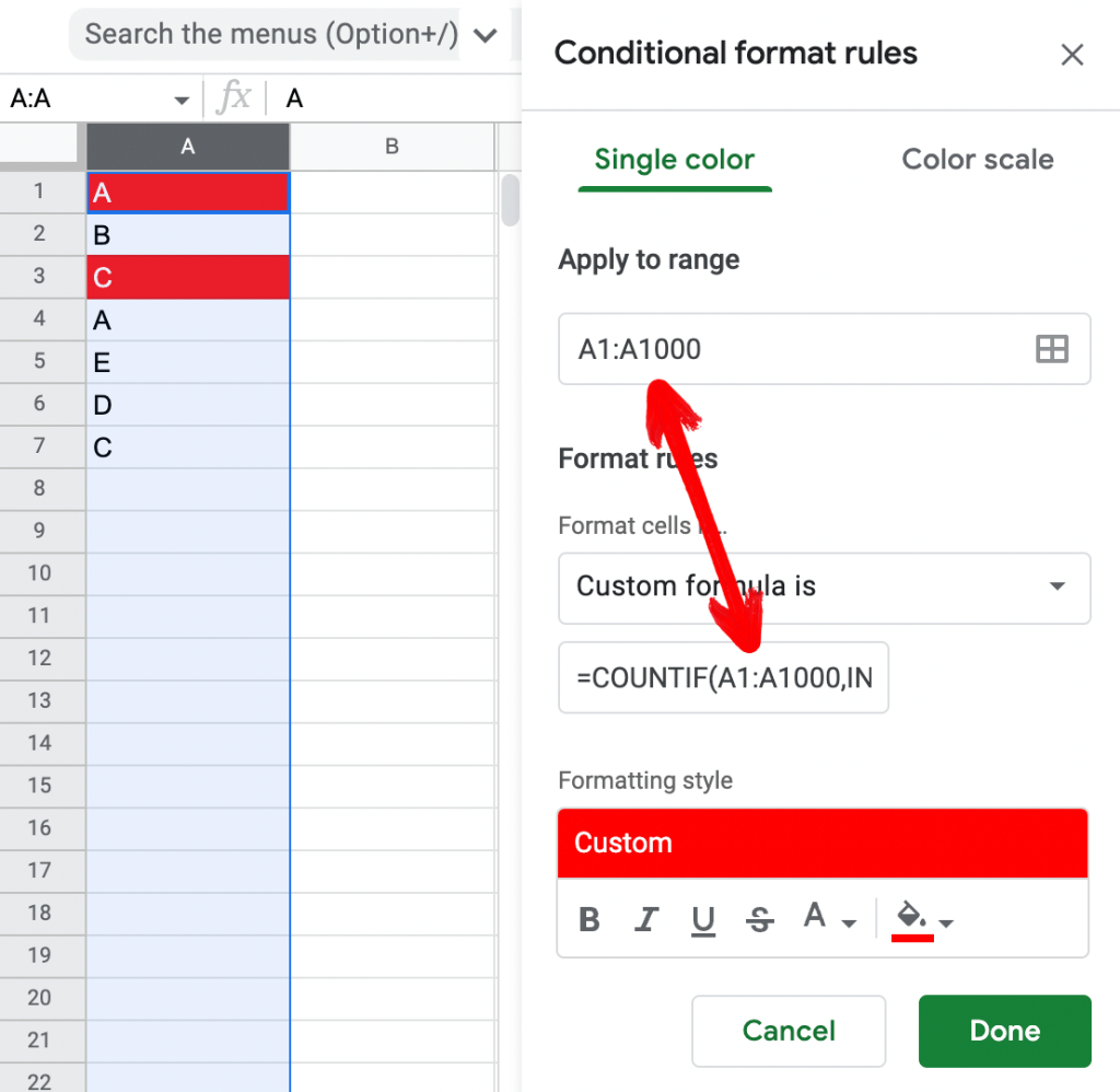
As you can see from the above example, the range in the Custom formula is section references the same range in the Apply to range section. This is important for the custom formula to work.
This formula works well with any type of range. Above a single column was highlighted, but the same could be applied to a row or a rectangular range.
Can the same formula work with multiple non-joining ranges?
Highlight Duplicates In Multiple Non-Contiguous Ranges
How can you highlight duplicates in ranges that are not joining?
The same formula is used, however, for each range, you would need to perform one slight change: you need to use INDIRECT for each range (whether named or not).
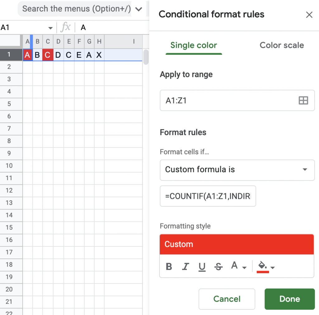
If I had a rectangular range from C3:F5 and wanted to keep the top row from A1:Z1 and see if both ranges contained duplicates my new formula for checking these ranges would now look like this:
Each range you would want to check again would need to be defined in its own COUNTIF function, with every range wrapped in the first parameter with INDIRECT("range").
You could make it easier by naming the ranges, like so:
Here’s the result of applying the above formula to the two ranges which are not connected or joined (I’ve highlighted the entire sheet to show that conditional formatting custom formulas will be needed in both the ranges):
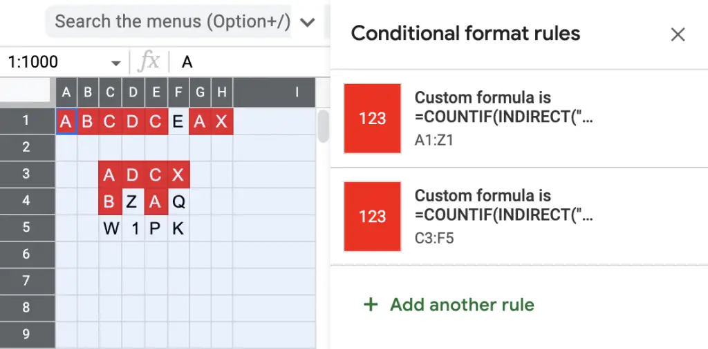
As you can see from the result, the highlighted cells which can be found in both the top row and the rectangular ranges are highlighted.
Summary
To highlight cells that are duplicated in a range, use the conditional formatting custom formula functionality with the formula =COUNTIF(range, INDIRECT("RC",FALSE))>1 where range matches the highlighted range applied for the conditional formatting.
If you want to highlight duplicates in non-contiguous ranges modify the formula slightly by making the formula: =COUNTIF(INDIRECT("range"), INDIRECT("RC",FALSE)) + ... > 1 where range is the range you want to check for duplicates and the ... representing the repeated formula again for each contiguous range. For example, =COUNTIF(INDIRECT("A1:Z1"), INDIRECT("RC", FALSE)) + COUNTIF(INDIRECT("C3:F5"), INDIRECT("RC", FALSE)) > 1 and this formula being pasted in each custom formula’s conditional formatting range (i.e. in ranges A1:Z1 and C3:F5).
By highlighting duplicates in your ranges you’ll be better able to warn users if they have accidentally typed a value that needs to be unique.