Conditional Formatting With Custom Formula Using Relative References

How can you apply conditional formatting using a custom formula that contains a relative reference to an adjacent row or column in Google Sheets?

If you want to highlight a cell in Google Sheets using conditional formatting based on the condition of a nearby cell you can easily do so by using the Custom Formula feature along with the INDIRECT() formula that contains a relative reference.

The INDIRECT(cell_reference, is_A1_notation) formula in Google Sheets contains two parameters with the first parameter being a string representing the specific cell reference either as a named range (i.e. salesTax ), or an absolute reference known by the common A1 notation with column letter followed by the row number (i.e. A1 ). The second parameter to the INDIRECT formula is_A1_notation is by default set to TRUE , therefore, when using a relative reference this parameter needs to be set to FALSE .

Here are some examples demonstrating each type of INDIRECT() formula call in a spreadsheet (cell B1 is a named range cell labelled as salesTax ):

	A	B
1	100 =INDIRECT("salesTax")	100
2	ABC =INDIRECT("B2")	ABC
3	A1B2 =INDIRECT("R1C2", FALSE)	A1B2

As you can see from the above spreadsheet snippet the INDIRECT() formula is used in three distinct ways with the first showing how to use a named range salesTax which references cell B1 , and the second showing an absolute reference using the A1 notation of "B2" , and the third using relative referencing.

What Is A Relative Reference?

A relative reference is the opposite of an absolute reference. An absolute reference is a reference specifically pointing to a range that is either named (i.e. salesTax ) or written in A1 notation. In contrast a relative reference cell is a reference to a range that is a specific number of rows or columns away from the active cell.

As demonstrated above in the spreadsheet snippet the last INDIRECT() formula contained a reference using the letters R and C along with a number alongside each letter. Instead of knowing the name of the cell or the exact A1 notation you can obtain the value of the cell using a relative reference to the cell needed.

The instructions needed to get to the cell require you to know the distance from the active cell to the cell you want to reference. The distance must be measured in rows (up, as a positive number, or down, as a negative number) and columns (right, as a positive number, or left, as a negative number).

Therefore compared to the absolute cell references the syntax used with a relative reference must contain an annotation in row distance and column distance .

The way this is designated in Google Sheets is by using the R label for row distance and the C label for column distance with adjacent to each label a number in square brackets of the relative distance from the active cell.

R[n]C[n]

relative reference syntax

For example, the relative reference of R[2]C[2] (which has nothing to do with R2D2’s cousin) from the active cell A1 may indicate the cell to increase the row by 2 values and to increase the column by 2 values.

If you think this would reference C3 you would actually be wrong . Why?

One major detail about the relative reference syntax is that the active cell has the relative reference R[1]C[1] . This could also be written as R1C1 or even RC .

Therefore, when using the relative reference R[2]C[2] in effect you are only increasing the row by one (not two!) and the column reference by one (not two!). The relative reference will point to cell B2 , not C3 .

If you wanted to reference a row above the active cell or to the left of the active cell then you can use a negative number in square brackets to obtain the value of cells above (where you need to reduce the row value) or to the left of the active cell (where you need to reduce the column value of the cell).

What happens when you use the relative reference R[-1]C[-1] in cell A1 ?

#REF! Error When Using Relative Reference

If you get a #REF! error when using a relative reference it could be due to two main factors:

You’re referencing a cell that cannot be found on the sheet. For example, if you’re in cell A1 and are referencing a row above the active cell, or referencing a column to the left of the active cell then because you are in the top and right-most cell there are no cells above and to the left.

Hence the #REF! error.

Another common reason for the #REF! error could be due to a circular reference . This could be the relative reference pointing to a cell which uses the active cell to help calculate its value, or you have entered into the relative reference any of the following values which indicate the active cell:

• R1C1
• R[-1]C[-1]
• RC1
• R1C
• RC
• R[0]C[0]

All of the above relative references mean the same active cell .

Relative Cell Reference With Conditional Formatting

With the basics understood of what a relative reference looks like and how it behaves in Google Sheets, you can now use this syntax in your conditional formatting.

Knowing how a relative reference works in Google Sheets can help with a conditional formatting range where you might want to highlight an entire row or column based on a cell in the row triggering a condition.

For example, if you wanted to highlight an entire row based on whether a value in the row is greater or less than some other value you can use the relative reference with the INDIRECT formula.

First, select the entire sheet and then click on the Format main menu then click on Conditional Formatting option.

From here create a new conditional format and select Custom formula is for the condition.

In the custom formula field enter the formula:

=INDIRECT("RC2", FALSE) > 1000

This formula means that if the value in the second column across (to the right) is greater than the value of 1000 then perform the formatting.

This would look something like this:

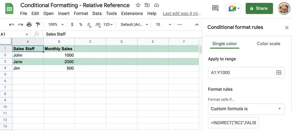
Notice for the highlighting to work the range must be over the whole sheet, in my case above A1:Y1000 . As the first header row is meeting the condition I would change the Apply to range cell to A 2 :Y1000 to have it ignore the first row.

However, as you can see the relative reference works in highlighting the entire row where the condition is met (i.e. where the monthly sales column is greater than 1000).

Highlight If Formula Does Not Exist In Cell

Another very popular conditional formatting technique I use is to check if a formula exists within a cell. This formatting can be very useful when you have important formulas and users tend to insert rows of data without knowing they need to copy the formulas in adjacent rows above.

With the same example of monthly sales staff if I added a column labelled Quarterly Sales that contained a simple formula of checking if the monthly sales value was present and if so to multiply that by 3, the formula would look something like this:

=IF(LEN(B2),B2*3,)

And I’ll copy this formula all the way to the end of the column. The sheet now looking like this:

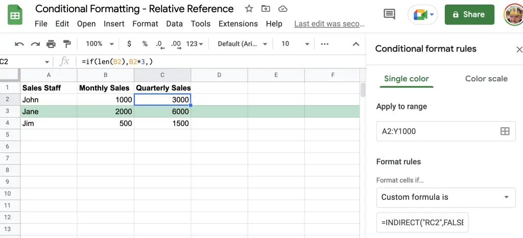
To make sure a user of the spreadsheet doesn’t come in and insert a row of data and forget to apply the formula you can use the ISFORMULA() formula on the active cell relative reference.

To add this type of conditional formatting to your spreadsheet simply highlight the range where a formula should exist and in the Custom formula is field enter the following formula:

=NOT(ISFORMULA(INDIRECT("RC", FALSE)))

This should look like the following in your conditional formatting area on your spreadsheet:

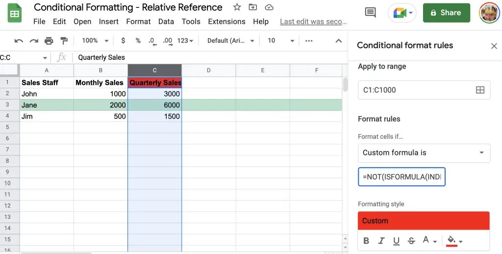
As you can see from the above screenshot the top cell is highlighted in red as it does not contain a formula, whereas the rest of the column is not as they all contain the quarterly sales projection formula.

Knowing that the header row will not contain a formula I can change the range from C1:C1000 to C 2 :C1000 to remove the conditional format applying to the header row.

Relative References: Summary

Conditional formatting can be a great way of being able to highlight and show the reader conditions being met, or something not being quite right. Knowing how to use relative referencing can help highlight an individual cell in a range, such as a cell not having a formula, or can be used to highlight an entire row.

Remember when using relative referencing in a conditional format to use the INDIRECT("R[n]C[n]", FALSE) formula where R[n]C[n] relates to the relative cell reference from the active cell.

If you’d like to see another conditional formatting example check this article where a custom formula based on a value in the first column is used to highlight the entire row .