How can you highlight an entire row based on a single condition in another column?
To highlight an entire row based on a value in a column using conditional formatting requires using the INDIRECT() formula.
A spreadsheet contains the following simple data where the first column contains a list of dates and the other columns contain corresponding data for that date.
Here’s a snapshot of the spreadsheet which contains Date, Bank Pmt Id and Interest Rate:
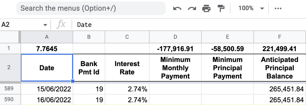
The simple spreadsheet has a payment schedule for each calendar day of the year and the corresponding interest charge, rates, principal amount and balances.
To highlight an entire row to check how the repayments are going a conditional format was placed on the entire sheet.
To do this, first highlight all cells in the active sheet.
Then click on the menu item Format then Conditional formatting.
With the conditional formatting sidebar that pops up click on the first dropdown menu labelled Format cells if... and select Custom formula:
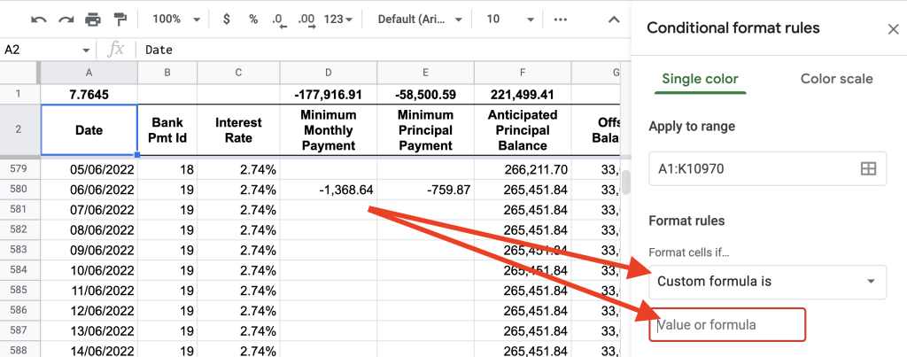
Click on the dropdown box which should enable you to enter a custom formula in an input box
As previously taught regarding conditional formatting and custom formulas the principles from this article help in easily creating a formula matching the requirement.
The custom formula is:
The custom formula for the conditional format contains two INDIRECT() formulas. The inner INDIRECT("RC", FALSE) formula represents the active cell as it loops through the entire highlighted range.
The outer INDIRECT("A"&ROW(x)) formula references the required first column for each row so that the comparison can be made.
Finally, the condition x=TODAY() checks if the value in column A matches today’s date. If this is TRUE then the conditional formatting will apply the formatting set.
Here’s how the spreadsheet looked:
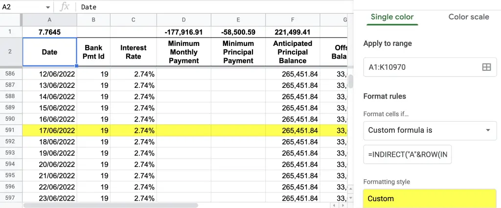
The custom formula works by highlighting the entire row as it matches today’s date
As you can see the custom formula inserted into the custom formula input box produces the highlighted row as it matches today’s date (don’t use NOW() as this includes time).
Summary
To create a conditional format that highlights an entire row based on a column in that range meeting a specific condition use the INDIRECT() formula to first grab the active cell (using INDIRECT("RC", FALSE)) and then use that in an outer INDIRECT() function to reference the specific column name along with ROW(x).
As the condition for this specific requirement was to have the first column in the sheet match today’s date the custom formula ended up being: