Google Sheets QUERY: Merge Multiple Columns & Expand Into New Structure (Example)

How do you merge multiple columns and then expand them into a different arrangement using Google Sheets?

Using a working example I will demonstrate how to migrate a specific data set containing columns, into a different data set using a different arrangement of columns.

The final formula is quite the monster and I’ll dissect this piece by piece to help demonstrate the process:

=ARRAYFORMULA(SPLIT(ARRAYFORMULA(SUBSTITUTE(TRANSPOSE(SPLIT(JOIN(" ",QUERY(DataConcat!A:L,,ROWS(DataConcat!A:A)))," ")),"~"," ")),";",TRUE,FALSE))

Original Data Structure

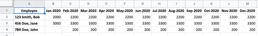
I had exported the following salary data from our budgeting software which contained how much each staff person would be receiving each month throughout the financial year.

An example of the raw data looked something like this:

Employee	Jan-2020	Feb-2020
123 Smith, Bob	2,000	2,200
456 Doe, Jane	3,000	3,300
789 Doe, John		200

Original structure of data

The original spreadsheet had all months of the year and I’ve labelled this import of data as Data in a new Google Sheet:

Employee Salaries — Employee salaries per month

Required Data Structure

Knowing what you have is one thing, but knowing what you need is the next important thing.

As I had to import this data into another application using CSV, it requires the following structure:

Employee ID	Employee Name	From Date	To Date	Amount
123	Smith, Bob	1/01/2020	31/01/2020	2,000
123	Smith, Bob	1/02/2020	29/02/2020	2,200
456	Doe, Jane	1/01/2020	31/01/2020	3,000
456	Doe, Jane	1/02/2020	29/02/2020	3,300
789	Doe, John	1/02/2020	29/02/2020	200

Data structure required to enable successful import into another application

As you can see with the requirements of the task, I need to be able to expand the data set to rows (as it’s currently laid out in columns), then merge the data back into one columnar set.

Thankfully Google Sheets makes it easy to export a sheet to CSV once I’ve achieved this result – simply use the handy File > Download > Comma-separated values (current sheet) option from Google Sheets’ main menu.

Step 1: Expansion

The first rule when manipulating data is to leave the original data set intact. This helps should there be an oopsie discovered later and you need to start from scratch again.

Therefore, I created a fresh new sheet and labelled this whatever was appropriate for my needs. In this example I will name it appropriate to what I’m doing: DataExpand .

In our expansion, we want to try and achieve all the required fields. This means I need to fetch the ID number from the original Employee field, and copy the remaining data into another field for the Employee Name . Then I’ll split the header column in the original sheet to a data range. Followed lastly with the amount in each date range.

My first sheet should look a little something like this:

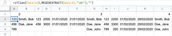
Expand Employee Salary — Perform the CSV requirement to get each ID on a separate row, and the employee name in a separate column, then break up each earnings into a start and end date per month

Here are the details as displayed in the photo above:

Cells $B$1 and $G$1 contained the =COLUMN() reference to each of the months on the original data set. This just helps with creating an easy index function that uses that reference which can make it easier copying the same columnar set 12 times.
Row 1 this contains the following formula to extract the ID number from the Employee field. Here I check to make sure I have data in the original Data sheet, if I do I want to perform a regular expression where I just want all the d igits, therefore, I used the regular expression of d+ :

=if(len(Data!A2),REGEXEXTRACT(Data!A2,"d+"),"")

From $B$2 down I then use another regex formula to extract those digits and replace them with nothing. I also want to check if the employee received any salaries or wages, if they didn’t I don’t want to add them into the data set.

=if(index(Data!$1:$1000,row(),B$1),trim(regexreplace(Data!$A2,"d+","")),"")

From $C$2 down I inserted the ID that is needed for each row if I have a confirmed value in the previous column.

=if(len(B2),$A2,"")

For $D$2 down if I have a value in $B$2 then I get the value of the salaries for that respective month. I use the handy index function here to get that value:

=if(len(B2),index(Data!$1:$1000,row(),B$1),"")

For $E$2 down if I have a value in $B$2 then I get the column heading of the respective month using, once again, the index function:

=if(len(B2),index(Data!$1:$1000,1,B$1),"")

Lastly, for $F$2 down I get the value in the previous cell, if something exists, and calculate what the last day of the month will be for that cell:

=if(len(E2),date(year(E2),month(E2)+1,0),"")

As I have been mindful of the formulas used for each budget month, I now need to copy cells $B$2:$F$1 and then paste this 12 times across. I could make it even easier by, after our first paste in cells $G$2:$K$4 changing cell $G$1 to be a formula: =$B$1 + 1 :

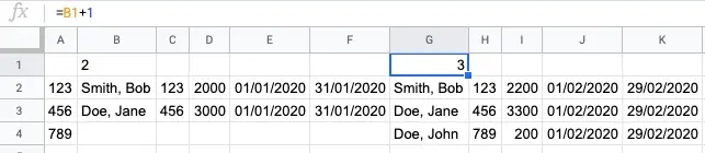
Then I copy this newly pasted range with formula edits across 10 more times.

Step 2: Concatenation

The purpose of the next sheet is to zip up our columnar collections. This is a relatively simple step, however, there are a couple of things to be wary of:

Use TEXTJOIN when zipping up the columnar data rather than the JOIN or CONCATENATE functions. The primary reason for this is where there is no data in a cell TEXTJOIN creates the blank join, whereas the other functions neglect it. As an example, if I had the following table:

	A	B	C
1	Missing	Puzzle	Piece
2	Missing		Piece

When using =JOIN(",",A1:C1) it produces the result Missing,Puzzle,Piece for the first row and =JOIN(",",A2:C2) will produce Missing,Piece for the second row.

Whereas using =TEXTJOIN(",",FALSE,A1:C1) produces the result Missing,Puzzle,Piece for the first row and =TEXTJOIN(",", FALSE, A2:C2) will produce Missing,,Piece for the second row.

As the TEXTJOIN function allows for the flexibility of the concatenation of your columnar data it’s import the data remain as it is represented elsewhere if there happen to be blank cells in your data.

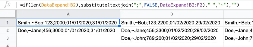
The other important aspect of this formula is that we want to replace the space characters within our cells as the space character will be used to join and split data back into columns again later. Therefore, it’s important at this step (if your data also contains spaces) to replace the space character with an oblique character that is not used anywhere in your data set.

I am going to replace my space characters within my data with the tilde character ~ .

Therefore, I have created a new sheet, which I’ve labelled DataConcat and cell $A$1 has the formula:

=if(len(DataExpand!B2),SUBSTITUTE(TEXTJOIN(";",FALSE,DataExpand!B2:F2)," ","~"),"")

Be mindful when transferring the data across to adjacent columns that you don’t copy-paste or drag across the formula, as each column here needs to reference the collection in DataExpand . For example, in the next adjacent cell $B$1 the formula is:

=if(len(DataExpand!G2),substitute(textjoin(";",FALSE,DataExpand!G2:K2)," ","~"),"")

You will need to do this 12 times for each month.

TEXTJOIN formula — Combine your data ready for merge using TEXTJOIN and SUBSTITUTE (if needed)

Step 3: Merge

So here’s where we merge all the columns from the DataConcat sheet in Step 2 above into one big column collection.

=ARRAYFORMULA(SPLIT(ARRAYFORMULA(SUBSTITUTE(TRANSPOSE(SPLIT(JOIN(" ",QUERY(DataConcat!A:L,,ROWS(DataConcat!A:A)))," ")),"~"," ")),";",TRUE,FALSE))

Wow, what a massive formula!

As with mathematics, I will start with the innermost functions and work my way out. So let’s break up each component within this formula and explain what’s happening:

`QUERY` function

QUERY(DataConcat!A:L,,ROWS(DataConcat!A:A))

Here we use the QUERY function to capture the data we want to operate on (the first parameter), being all the columns in the DataConcat sheet, and we then want to combine these cells into one row. We achieve this by setting the number of headers (the third parameter) to the maximum number of rows in the DataConcat sheet. This means every row in the DataConcat sheet will be zipped up into one row!

The way the QUERY function zips everything up is by applying the space character to each new cell. This was why it was important for us to remove the space characters from our own data set before we applied this function .

If you’d like to know more about the QUERY function I wrote up a more detailed post here explaining this type of use.

MERGE – Using `JOIN` , `SPLIT` & `TRANSPOSE` functions

TRANSPOSE(SPLIT(JOIN(" ", QUERY(...)), " "))

The combination of these three functions is to merge the single row returned by the QUERY function into one column.

First we JOIN the rows together using the special space character which helps to delimit each individual row. Then we SPLIT by the space character which produces the rows across individual cells horizontally. Finally, the TRANSPOSE function translates the horizontal cells into vertical formation – a single column.

Unfortunately the JOIN function does have a character length limitation of 50,000 characters. You may need to break up your requirements or look at other means if this ends up being an impediment.

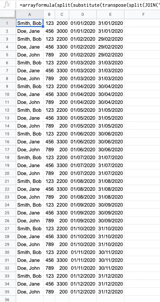
EXPANSION – Using `ARRAYFORMULA`

The last step is to expand our singular column so that it can be represented as needed for CSV export. If we’re expanding data sets we need to use the ARRAYFORMULA function, as demonstrated here:

ARRAYFORMULA(SPLIT(SUBSTITUTE(transpose(...), "~", " "), ";", TRUE, FALSE))

The ARRAYFORMULA provides us with the ability to loop through each of the cells in our data set and to apply individual functions to them. In our case, we want to:

SUBSTITUTE back the oblique tilde ~ character with its original space character.
SPLIT back the data we concatenated in the DataConcat sheet. However, we need to be mindful there may be instances where we have blank cells, and we want the SPLIT function to return the blank cells, therefore, we need to change our fourth parameter in the SPLIT function to FALSE (default is TRUE ). By switching this to FALSE it turns consecutive delimiters like ;; into three separate cells, rather than just one cell.

With these functions all combined, they produce the outstanding result intended, like so:

ARRAYFORMULA function — Expansion of our singular column using `ARRAYFORMULA` , `SUBSTITUTE` and `SPLIT`

Summary

Within this post, I learned how I can extrapolate data from one form to another using several intermediary steps and complex Google Sheet functions.

Hopefully, this post has been helpful with learning:

How to organise your steps by leaving the original data set (use multiple sheets if needed).
How to use the QUERY function and especially its third headers parameter.
Why you would use the TEXTJOIN function over JOIN .
The limitations of the JOIN function.
How to expand your data set using ARRAYFORMULA with any function when needing to loop through individual cells in the result.
How to set the SPLIT function’s fourth parameter so that consecutive empty cells aren’t treated as one.