If you have two or more columns of data and you want to merge these columns into one column then using the Google Sheets
QUERY
formula may be one way you can achieve this.
Here’s an in depth explanation of how to achieve this:
Step 1 – Prep your data
If you data doesn’t contain any spaces then you’re good to go, if though your data does contain spaces then you will need to define a character at the end of each cell to get this to work.
Step 2 – Understanding the
QUERY
Function
Let’s have two simple data sets, one which does not contain spaces in its data set, and another which does:
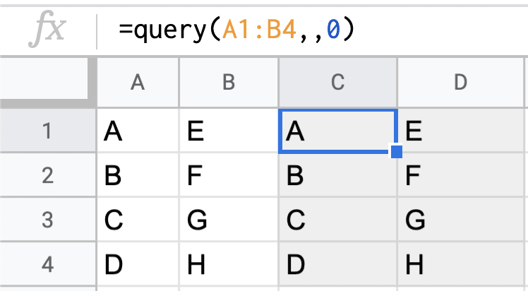
QUERY
function with no header

QUERY
function with no header
With both data sets, we have highlighted in grey the returned values from the
QUERY
function.
QUERY()
parameters
The
QUERY
function is a powerful formula in Google Sheets helps to treat data contained in tabular format like a database table which we can perform basic
SQL
queries on.
This function contains three parameters:
- The data set.
-
The
SELECTcommand. - The number of headers in your data set.
It’s the third parameter of the
QUERY
function that will help us in being able to concatenate the data within each column.
At the moment, from above, we have set the third parameter to
0
which means our data set does
not
return any headers.
But what if I want to define the first row as being the header?
Then we would simply change this third parameter in the
QUERY
function to
1
– representing the first row. When we perform this change to our formula we see no change to our data, however, the returned values have now defined that first row as a header area.
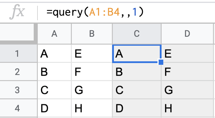
QUERY()
Header Parameter
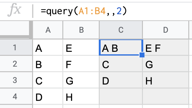
What if we were to increase the number represented in our
QUERY
function? How is the result set returned if we define the
header
parameter as
2
?
Here’s how it looks for our data sets:
Did you notice what the
QUERY
function does when we define more than one header row?
It concatenates the header rows and inserts a space between each appended element. Therefore, the first row containing
A
and the second row containing
B
produce the header
A B
.
(Can you foresee the issues we’re going to run into when we merge our columnar data which contains spaces already?)

So if we wanted to get all the elements within our column wrapped into one row we would just need to change that third parameter to the maximum height of our columns. We could use the
ROWS()
function to capture this number:
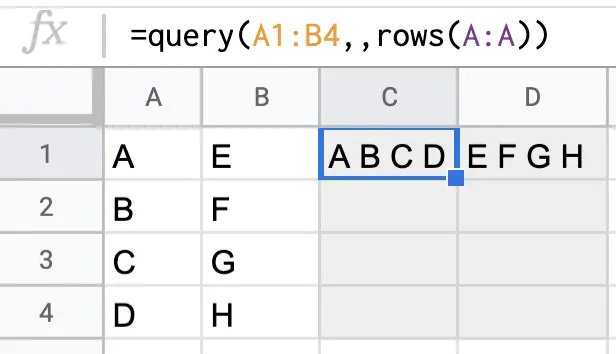
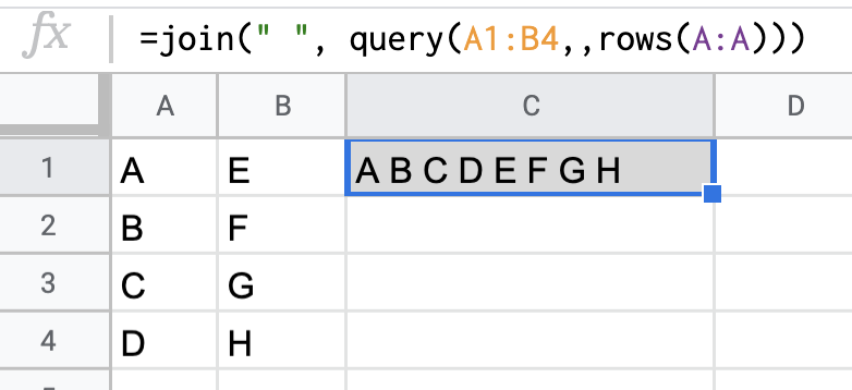
Step 3 – JOIN columns
As the columns have been merged into one header row, we now want to stitch these column headers together.
This is achieved by wrapping the
QUERY
function in a
JOIN
function, like so:
JOIN
query header rows together to combine into one cell
Notice here we used the first parameter of the
JOIN
function as a space to mimic the behaviour of what the
QUERY
data did to our data too.
Do be aware the
JOIN
function does have a limit of
50,000
characters. If you have a lot of data to concatenate you might want to break it up to smaller data sets.
What if our data contains spaces?
As you can see this strategy isn’t going to work too well as our result now contains too many spaces between data cells, and looks as follows:

Therefore, we’re going to need to improvise on the spaces in our current data set.
What we’re going to do is to modify our original data by substituting spaces for an oblique character that isn’t used in our data. For example, my current data set with names isn’t likely to have a tilde character
~
.
Therefore, what we want to be able to do is to change our imported data set in the
QUERY
function so that we are operating on data that doesn’t contain any spaces – we want to be able to reserve these spaces for the explicit purpose of being able to split our data back into cells again.
One such way I achieved this was by changing our original formula:
QUERY(A1:B3,,ROWS(A:A))To this:
QUERY(ARRAYFORMULA(SUBSTITUTE(A1:B3," ","~")),,ROWS(A:A))
What has happened with our first
QUERY
parameter?
Instead of referencing the original data set we modify the data set to substitute spaces for our oblique tilde
~
character.
The
ARRAYFORMULA
provides us the functionality of being able to operate on
each
cell within the range, and all we want to do is apply the
SUBSTITUTE
formula to each cell – if it has a space character replace it with the tilde character.
The result of our change should produce something like this:

ARRAYFORMULA
and
SUBSTITUTE
We’ve now achieved our purpose of reserving the space characters for another specific purpose which we’ll see next.
Step 4 – Transform back to one column
Our data is in one cell, split by the space character.
To stretch this back out into one single column all we need to do is
SPLIT
the data by the special space character and then
TRANSPOSE
it to leave the data as a column, otherwise it will remain in row fashion if we don’t.
Here’s what happens to our first data set when we
SPLIT
first:
=SPLIT(JOIN(" ", QUERY(A1:B4,,ROWS(A:A)))," ")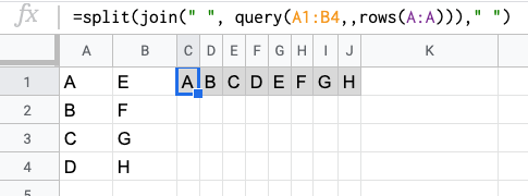
SPLIT
data after
JOIN
&
QUERY
functions
Then our concluding formula for the first data set:
=transpose(split(join(" ", query(A1:B4,,rows(A:A)))," "))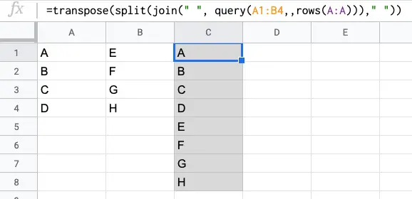
TRANSPOSE
data after
SPLIT
,
JOIN
&
QUERY
What about our data set with spaces?
A little more work is going to be required with our original data set which contains spaces.
If we copy the above formulas into our working “space” formula here’s the result:
=TRANSPOSE(SPLIT(JOIN(" ",QUERY(ARRAYFORMULA(SUBSITUTE(A1:B3," ","~")),,ROWS(A:A)))," "))
TRANSPOSE
and
SPLIT
formulas
As you can see we need to remove at the end each of those tilde characters.
How do you think we could do this?
If you were thinking
ARRAYFORMULA
and
SUBSTITUTE
again – well done! You’re acquiring a new skill today.
Here’s our concluding formula:
=ARRAYFORMULA(SUBSTITUTE(TRANSPOSE(SPLIT(JOIN(" ",QUERY(ARRAYFORMULA(SUBSTITUTE(A1:B3," ","~")),,ROWS(A:A)))," ")),"~"," "))
QUERY
function.
Summary
So there you have it!
Within this article you’ve been able to learn the following function skills when using Google Sheets:
-
What the third parameter of the
QUERYformula does. -
How we can modify each cell within a range by using
ARRAYFORMULA– specifically using theSUBSTITUTEformula. -
How to handle different data sets with the
QUERYfunction, especially if they contain space characters. -
How to
JOINourQUERYdata to form a single cell of data (careful of the 50,000 character limit). -
How to
SPLITour data set back into cells. -
How to
TRANSPOSEour data set back into columns.
Well done if you’ve been able to follow along and understand these complex topics.
