What Does $A$1 Mean In Excel Or Google Sheets?

What does $A$1 mean in a spreadsheet formula in Excel or Google Sheets?

The syntax $A$1 is simply an absolute reference to cell A1 .

The reason why there are dollar signs prefixed in front of the column and row labels is to prevent the cell from changing its reference as the original cell is copied to another cell.

If a cell containing a reference to A1 is not needed to be copied, or if the reference to cell A1 is not needed to be fixed when copied elsewhere, then the dollar signs are not required.

Fixing Reference To Cell A1

The primary reason why you would want to make a cell reference absolute is that the formula needs the value contained in cell A1 and if the cell with the formula containing the reference to cell A1 is either copied or moved this reference will not change.

Here’s an example demonstrating what would happen if I copied the cells with formulas in column B across to column C :

	A	B	C
1	2022	2024 =$A$1+COLUMN()	2025 =$A$1+COLUMN()
2		2024 =A1+COLUMN()	2027 =B1+COLUMN()

As you can see the values in column C for the first row contain the same formula (though they have different values due to the changing value of the COLUMN() formula). Whereas the value in the second row have different values when comparing cell C1 to C2 because cell C2 does not have an absolute reference to cell A1 , instead it changes across with the direction of the copy and moves the column reference across to cell B 1 .

If cell B1 were copied down to cell B3 what would happen to the formulas cell reference to A1 ? This would change the row reference from A1 to A 2 as shown below:

	A	B	C
1	2022	2024 =$A$1+COLUMN()	2025 =$A$1+COLUMN()
2		2024 =A1+COLUMN()	2027 =B1+COLUMN()
3		2 =A2+COLUMN()

As the reference in the formula in B3 has changed to A2 which is an empty cell this equates to the value of 0 and the COLUMN() formula is 2, therefore 0 + 2 = 2 .

Whereas if we copied cell B1 down to cell B4 this would be the result of that operation:

	A	B	C
1	2022	2024 =$A$1+COLUMN()	2025 =$A$1+COLUMN()
2		2024 =A1+COLUMN()	2027 =B1+COLUMN()
3		2 =A2+COLUMN()
4		2024 =$A$1+COLUMN()

As you can see from the above formula that was copied from cell B1 to B4 the result is the same (as the copied cell is in the same column). While the formula COLUMN() will change depending upon where you copy it to the absolute reference $A$1 stays the same.

Absolute Reference Keyboard Shortcut

To make it easier to enter an absolute reference for a cell in your Google Sheets you can use the shortcut key F4 to have the spreadsheet automatically insert the necessary dollar signs for the active range your cursor is active on or have just typed in your formula.

For example, if you have just started typing the following formula and your cursor is at the end of the cell reference A1 as shown below:

=A1│

In Google Sheets you can then hit the F4 function key on your keyboard and this will change the formula to the following:

=$A$1│

If you continue tapping the F4 key on your keyboard it will cycle through all the different types of absolute references available for the active range in your formula, therefore, next will be:

=A$1│

This absolute reference keeps the row label the same, and if the F4 key is tapped again then the absolute reference changes to:

=$A1│

This absolute reference keeps the column label the same, and if the F4 key is tapped again the user is returned back to their original cell reference:

=A1│

Therefore, if you do accidentally hit the F4 key on your keyboard and there is no need to make a cell reference absolute, you can continue tapping the F4 key to cycle back to your original reference without having to delete the dollar signs from your cell reference manually.

The order of the F4 keypress is as follows:

1. Both row and column absolute
2. Just row absolute
3. Just column absolute
4. No absolutes

This means if your cell already contains or is absolute that pressing the F4 key will step to the next sequence.

For example, if I have a cell reference that is already $A1 (column absolute only) and I tap the F4 key, the cell reference will change to the next sequence, being no absolutes, and will show A1 .

Does the F4 keyboard short cut also work with ranges?

Yes, the same F4 keypress also works if the last cell reference is part of a range.

For example, if you’ve just entered a formula that requires a range (like the SUM function) and the active cursor is at the end (or even anywhere in the range notation):

=SUM(A1:A2│

Hitting the F4 key on your keyboard will produce the same type of absolute references, but will apply the absolute references to the entire range , like so:

=SUM($A$1:$A$2│

The first F4 keypress will produce an absolute range, the second F4 keypress will produce an absolute reference on the row labels, like so:

=SUM(A$1:A$2│

And the third F4 keypress will produce an absolute reference on the column labels, like so:

=SUM($A1:$A2│

And finally the fourth F4 keypress will return the absolute references back to their original form:

=SUM(A1:A2│

Can you make just one cell reference in a range absolute using the shortcut key method?

No, you cannot. If you need to make an individual cell in a range absolute, you would need to insert the $ signs yourself manually.

Here’s what an absolute range reference would look like where only one part of the range reference is absolute:

=SUM($A$1:A2│

This reference above would mean the SUM range is increasing in size as the formula is copied either across or down.

However, if you do accidentally tap the F4 key, it will begin to make changes to the absolute references of the range. To return an absolute range reference back to what it was initially, just keep tapping the F4 key ( 4 times should do it ), and you will have your formula back as it was prior to the absolute references, here’s what the cycles looked like at each F4 keypress from the initial formula above:

1. =SUM(A$1:$A$2│
2. =SUM($A1:A$2│
3. =SUM(A1:$A2│
4. =SUM($A$1:A2│

As you can see from the above changes made by Google Sheets at each F4 keypress, the range is returned to its original form after 4 keypresses.

How To Reference $A$1 Without Dollar Signs?

If using the absolute reference syntax for a cell, aka the dollar signs, makes your formula difficult to understand there are two other alternatives available: use named ranges, or use INDIRECT formula.

What Are Named Ranges?

Every cell in a spreadsheet has a reference and this is commonly seen with alphabetic characters followed by numeric characters. For example, AA149 references the cell found at the intersection of cells in column AA and cells in row 149 .

However, cell references can be difficult to manage when you’ve got lots of them in a formula.

I prefer using named ranges whenever I have a formula containing more than a couple of absolute references. I find I can easily get things messed up when there are too many absolute references in one formula.

Therefore, instead of using absolute references you can change these cells (or ranges) to a named range .

To create a named range simply select the cell (or cells) and in the white area that contains the reference of the cell (or range) enter a name you would like to call it.

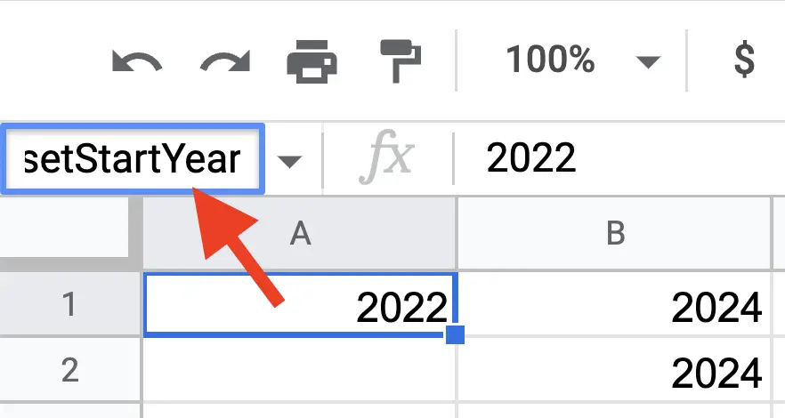
A type of nomenclature that I have adopted when naming cells that are referenced throughout the spreadsheet is to prefix the name of the cell (or range) with an abbreviation of the sheet. For example, if I have a Settings sheet and it has individual cells that reference specific details I would click on each cell and start the name of the range as setStartYear – if the cell was to hold the starting year.

I’ve found when you can adopt a naming system that makes sense for you it can be easy in knowing where to go to check the value of that cell AND it prevents name clashes.

Whatever strategy you adopt be mindful of naming clashes where two named ranges have the same name on different sheets. Some spreadsheets, such as Google Sheets, will allow you to have the same name, but the named range would need to be prefixed with the name of the sheet.

For example, Settings!StartYear if the named range StartYear was used on another sheet.

To me it kind of defeats the purpose of a named range if you have to prefix it with the reference of the sheet name, however, I’m doing this anyway – just in an abbreviated way!

Use INDIRECT Formula

If naming ranges doesn’t meet your taste then another option to consider would be the INDIRECT formula.

The INDIRECT formula takes two parameters: a cell reference (as a string), and a boolean value if the reference is in A1 notation (default for this parameter is TRUE if nothing is entered).

Therefore, instead of using $A$1 you could use INDIRECT("A1") .

As the reference contained within the formula is static (i.e. a string value pointing to a cell reference) it will not change when this formula is copied or moved.

The INDIRECT formula can also take a named range as its first parameter, i.e. using the named range setStartYear this would look like this with the INDIRECT formula: INDIRECT("setStartYear") .

At least if you’re unsure of which alternative to use you could use both!

Summary

The absolute reference $A$1 points to cell A1 in its formula. The dollar signs wrapped inside the reference merely fix the reference so that should the formula move or be copied the reference to A1 will not change.

If you find there are just too many dollar symbols in your formula, two alternative ways of using the absolute reference are to use named ranges or the INDIRECT function.

An easy way of making a cell reference absolute is to use the keyboard shortcut F4 , which when tapped multiple times will cycle through all the different forms of absolute cell references available for the range. If the cell does not have any absolute references the first F4 keypress will make both the row and column labels fixed, second F4 keypress will make the row label fixed (only), the third F4 keypress will make the column label fixed (only) and the fourth F4 keypress will return the cell back to it’s original form.

Overall, the absolute cell reference is used to fix or make constant a cell reference in a formula.