3 Ways To Make VLOOKUP Dynamic In Google Sheets (Examples)

How do you make the range and column index number in a VLOOKUP function in Google Sheets dynamic?

The VLOOKUP function is a popular formula used in spreadsheets to source data using the first column of a range as the primary key to search the search_key and then to return the intersection of the cell in that row with column_index_number.

Here is the syntax of the VLOOKUP function with its named parameters:

As stated above the first parameter search_key is the value in the range‘s first column you want to search, with column_index_number being the column to return from the row matching the search_key. The last optional parameter is_sorted can be set to FALSE to find an exact search for search_key, or TRUE to perform an approximate match of search_key.

(If using TRUE for is_sorted it is best to have your range sorted by the first column in ascending order to prevent getting a wrong return value.)

Knowing the parameters of the VLOOKUP formula can help to determine what aspects you want to make dynamic, and there are three parameters than can dynamically change:

• search_key this can change according to what you would want to search for;
• range this could change according to where you need to search; and
• column_index_number could change according to what value you want to be returned.

Changing the search_key value is trivial, so I’ll explore how to make the VLOOKUP function dynamic by modifying the second and third parameters in this article.

VLOOKUP Dynamic Ranges

There are multiple approaches to making the range dynamic with the VLOOKUP function. One approach is to use the INDIRECT function, which is useful when the search_key needs to be located in a different column. Another approach is to use the FILTER function, which is useful when the search_key can be found multiple times in the first column of the range.

Here are some examples demonstrating how each approach works.

Dynamic VLOOKUP With INDIRECT For range

As the second parameter in the VLOOKUP function requires a range to make this dynamic, you would need to use the INDIRECT formula.

One reason why you may want to make the range dynamic is to change the field for the primary key according to the type of search_key entered.

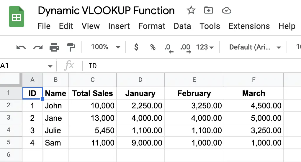
For example, if you have a Summary sheet containing the staff IDs, Names, Total Sales YTD and Sales for Each Month, you could make the range dynamic by using INDIRECT function according to the type of search entered for the staff member.

Here’s an example of what the Summary sheet would look like:

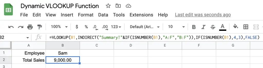
To construct a dynamic VLOOKUP range would mean creating a formula like so in a new sheet:

The result is the following when entering the name Sam in cell B1:

And here’s the same sheet where the search_key is an employee’s ID:

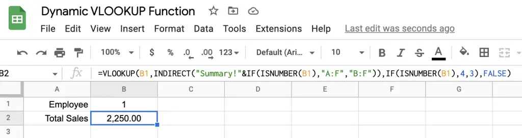
As you can see with both results, the desired outcome is achieved. However, when making a VLOOKUP formula dynamic when expanding or contracting the range width, you will need to make the column_index_number parameter dynamic too.

When the range of the VLOOKUP formula is modified in height, then the column_index_number can stay the same.

Dynamic VLOOKUP With FILTER For range

Another popular approach is to apply a filter on the range. This is common when the search_key can be found multiple times in the first column of the range.

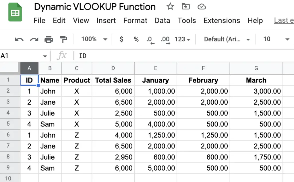
As the Data sheet contains more than the Summary sheet, for example, including the individual Products sold per month if a result was needed for the total sales made of a specific product the range would need to be compressed to just those rows.

Here’s what the Data sheet looks like:

Here’s how the formula would look when using the FILTER function combined with the VLOOKUP:

Here is how the sheet is constructed and it’s result:

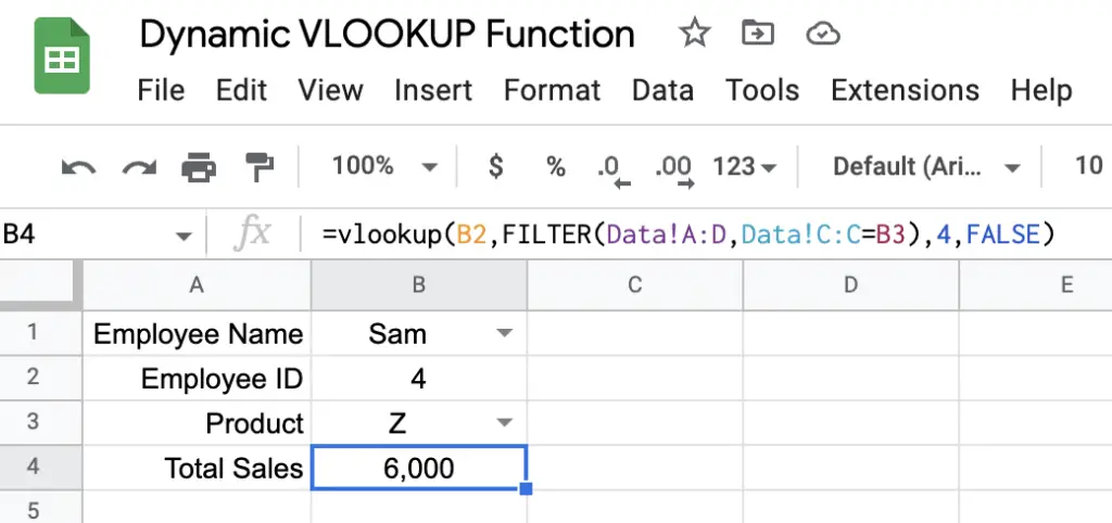
As you can see from the above result the FILTER function helps to reduce the rows in range by the conditions placed in the second and subsequent filters. In this case, the Data sheet is reduced by column Data!C:C matching cell B3.

VLOOKUP Dynamic Column Index Number

To make the index column in the VLOOKUP function dynamic, use the MATCH formula in the index column parameter. This approach is useful when specific data is needed from a specific column.

With the example spreadsheet used, if you wanted to obtain a specific total amount of sales for a specific month, then you can use the VLOOKUP formula with MATCH to obtain the specific intersection of the found search_key and the matched column index number.

Here’s how this formula would look:

Here’s how the result looks in the spreadsheet:

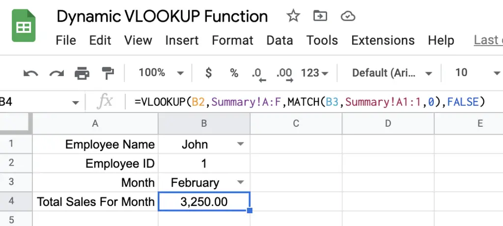
As you can see from the above, the result changes according to the input from the specific month requested. The MATCH formula finds the matching column name in cell B3 and returns the index where this item is found, which is what is needed for the column_index_number.

Instances where it helps to make the column_index_number dynamic will happen when you want to obtain a result from the intersection of the searched row and a specific column.

Summary

There are 3 approaches you can use to make the VLOOKUP function dynamic. One approach is to modify the range using the INDIRECT formula, which can be helpful when you want to change the field for the primary key according to the type of search_key entered. When using this approach you will need to modify the column_index_number if the returning column needs to stay the same.

Another popular approach is to apply the FILTER function to the range. This is common when the search_key can be found multiple times in the first column of the range, and the data can further be reduced by applying filters.

Finally, another way to make the VLOOKUP function dynamic is by changing just the column_index_number dynamic by using the MATCH formula. This approach is useful when specific data is needed from a specific column.

Click here for a free copy of Dynamic VLOOKUP Google Sheet