Google Sheets

How do you concatenate two ranges into one contiguous range for use in the QUERY function for the data parameter in Google Sheets? To concatenate two ranges into one for use as the first parameter in the QUERY function in Google Sheets, simply combine your data sets together using the set notation {} and the semi-colon character to separate each range ; e.g. {{Data!A:A, Data!B:B};{Data!A:A, Data!C:C}}. For example, suppose you have the following transactional data on sales and associated direct costs like so on a sheet labelled Data: ...

How do you reference a cell in the WHERE clause of a Google Sheets QUERY function? To reference a cell in the Google Sheets’ QUERY function WHERE clause, simply break the query string by closing with a double-quoted string " append the concatenation symbol & then reference the cell append the & to open up the query string again " so you can continue writing the rest of your query. Do be mindful it does depend on the type of value being referenced in the cell as well. If the cell reference is a string, you will need to make sure you wrap the cell reference in single quotes. ...

How can you apply conditional formatting on checkbox cells in Google Sheets? Conditional formatting in Google Sheets can be applied to a range of checkboxes by applying the conditional formatting condition of Is equal to to TRUE. Here’s an example demonstrating how to set a conditional format on checkboxes. Create Checkbox Range To create a range of checkboxes, select your range and then click on the Data Validation menu item. ...

How do you highlight duplicates in a defined range using conditional formatting in Google Sheets? To highlight cells that are the same value in a range, select the range and use a custom formula in the conditional formatting area that uses relative referencing. The custom formula you will want to insert into the conditional formatting area is: = C O U N T I F ( r a n g e , I N D I R E C T ( " R C " , F A L S E ) ) > 1 Where range is the same highlighted range of the conditional formatting range. ...

How can you extract a date from a string in a cell in Google Sheets using the powerful REGEXEXTRACT() function? The REGEXEXTRACT(text, regular_expression) function has two parameters with the first labelled as text being the string operated on and the second labelled as regular_expression being the regular expression (using RE2 syntax) to extract data from. Here are a few popular examples of how you can use this powerful function to extract dates from a string in Google Sheets. ...

How can you highlight an entire row based on a single condition in another column? To highlight an entire row based on a value in a column using conditional formatting requires using the INDIRECT() formula. A spreadsheet contains the following simple data where the first column contains a list of dates and the other columns contain corresponding data for that date. Here’s a snapshot of the spreadsheet which contains Date, Bank Pmt Id and Interest Rate: ...

What does $A$1 mean in a spreadsheet formula in Excel or Google Sheets? The syntax $A$1 is simply an absolute reference to cell A1. The reason why there are dollar signs prefixed in front of the column and row labels is to prevent the cell from changing its reference as the original cell is copied to another cell. If a cell containing a reference to A1 is not needed to be copied, or if the reference to cell A1 is not needed to be fixed when copied elsewhere, then the dollar signs are not required. ...

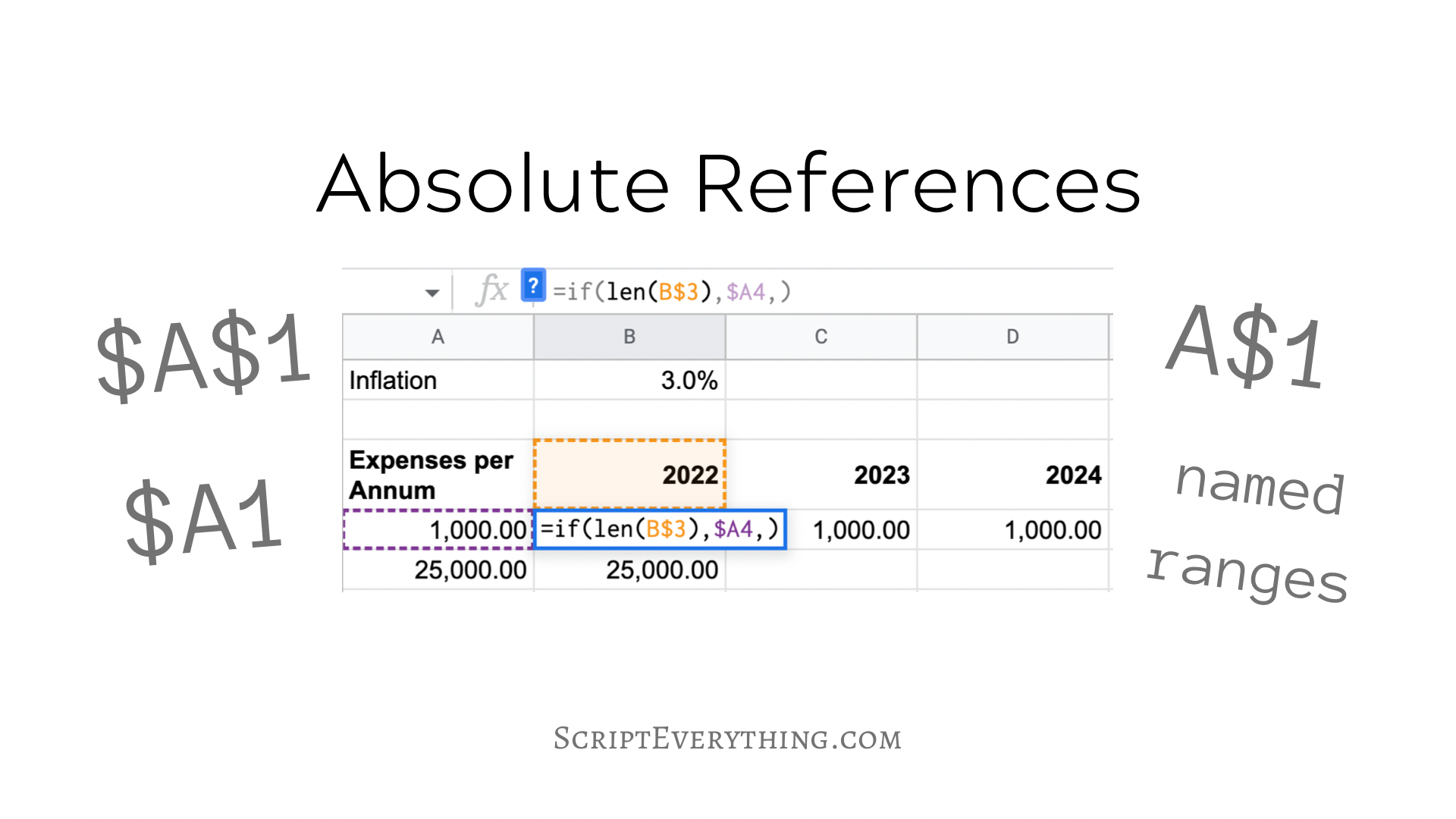
How do you use absolute cell references in a spreadsheet like Excel or Google Sheets? An absolute cell reference is a reference containing the common column letter and row number labels but around those labels are either one or two dollar signs. For example, the following references for cell A1 are all absolute references: $A$1, $A1 and A$1. What’s the difference between each of three references? The purpose of the dollar sign in front of the column label and/or the row label is that this fixes the column or label. This helps when copying a cell and you want the reference of the column or row or cell to remain static. ...

How do delete an attached Google App Script file and project from a Google Sheet? I recently wanted to copy a Google Sheet and as I did I noticed it had an attached Google App Script file. Here’s what that dialog window displayed: However, I didn’t want the adjoining scripts with the copy, in fact I wanted to delete all the original scripts from the original spreadsheet as these were no longer needed. ...

How can you apply conditional formatting using a custom formula that contains a relative reference to an adjacent row or column in Google Sheets? If you want to highlight a cell in Google Sheets using conditional formatting based on the condition of a nearby cell you can easily do so by using the Custom Formula feature along with the INDIRECT() formula that contains a relative reference. The INDIRECT(cell_reference, is_A1_notation) formula in Google Sheets contains two parameters with the first parameter being a string representing the specific cell reference either as a named range (i.e. salesTax), or an absolute reference known by the common A1 notation with column letter followed by the row number (i.e. A1). The second parameter to the INDIRECT formula is_A1_notation is by default set to TRUE, therefore, when using a relative reference this parameter needs to be set to FALSE. ...