How can you create a conditional format in Google Sheets based on the value from another cell or column regardless of whether that cell is on the same sheet or another?
To reference any cell or column in the Custom Formula field in Google Sheets’ conditional formatting section use the INDIRECT() function referencing that cell or adjacent column.
Recently I had a simple requirement where I wanted to highlight a range of cells according to the MONTH() of a cell containing a date value.
For example, I had a cell on a Settings sheet which I gave it the Named Range value of setEndDate. The cells I wanted to highlight had the name of the month and I wanted to highlight these cells that matched the month of the setEndDate field.
I knew my formula would initially look something like this, where A1 was the first cell in the selected range where I wanted the highlighting to start:
Remember when setting a Custom Formula the first cell needs to be inserted into the formula. Google Sheets then automatically replaces this cell reference with the next cell in the range where Conditional Formatting will apply.
This is a very important point as you’ll soon see why.
Here’s what happened when I inserted my formula into the Custom formula is field in the Conditional formatting section, as you can see it didn’t work:
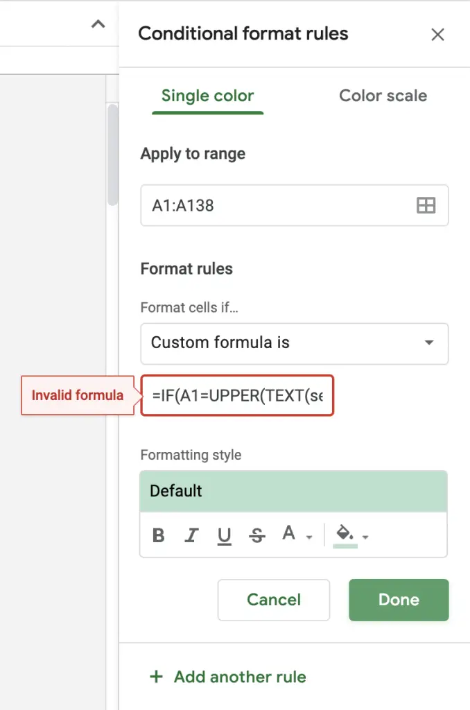
It doesn’t matter whether a Named Range value or the actual range reference (eg. Sheet1!A1) is inserted into the formula the result is still the same: Invalid Formula.
How To Get Around Invalid Formula Error With Cell References
To get around the Invalid Formula error in the Custom Formula field in the Conditional Formatting section simply replace the cell reference (whether an actual reference or Named Range value) by wrapping it into the INDIRECT() formula.
The INDIRECT() function translates the value inserted into the parameters of the function into a value that is used by the remaining formula, so my initial function changed to this:
And this enabled the Custom Function to work.
Conditional Formatting And IF Statement
The purpose of a Custom Formula used in a conditional format is to structure the formula so that it is a boolean operation. While you can use an IF() statement as above it needs to return boolean values so Google Sheets knows when to apply the format.
Therefore, if the IF() function is already returning boolean values and in the correct order (i.e. TRUE is the first value returned after the statement, and FALSE is the last value returned) then the IF() statement is redundant and can be removed.
My custom formula would now look like this:
If your IF() function has the boolean values swapped – i.e. IF(statement,FALSE,TRUE) then you still can remove the IF() statement and instead wrap your statement section with the function NOT().
For example, if I wanted to highlight cells that were not empty using a custom formula I could write the following:
This conditional format works on the range where it is applied (in A1:A138) and will highlight the cell if the cell is not empty.
The function NOT() simply reverses the boolean result inside. The original function inside states A1 is empty, therefore, should a cell be empty the NOT() function returns FALSE whereas if a cell is not empty, being FALSE inside, the NOT() function returns TRUE.
Why Use INDIRECT For Custom Formula?
The reason why the INDIRECT() function is needed in the Custom Formula is because of the replacement by Google Sheets of cell references when it applies the logic to other ranges in the Conditional Formatting range.
With my formula above you can see that there is one cell reference inserted into the formula, in my case, the cell A1:
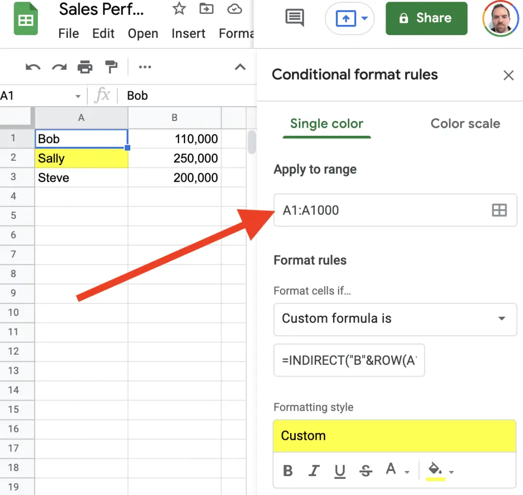
And the Apply to range field (as shown in the picture above) is set to A1:A138.
Therefore, when Google Sheets applies my Custom Formula to the next cell in my A1:A138 range it finds the only cell reference in the formula and replaces it with the next cell, therefore, A2 would look like this for my custom formula:
Hopefully, you can see why inserting more than one cell reference into a custom formula does not work, and the only way to get a formula to work where other cells are referenced is to use the INDIRECT() function.
Conditional Format Based On Another Column
What if there were data in an adjacent column as you tracked down the column you wanted to perform the conditional formatting? Can the Custom Formula use adjacent or same length columns to perform a comparison?
Suppose you have the following set of data in your spreadsheet which lists the total amount of widgets sold in a month per sales staff member:
| A | B | |
|---|---|---|
| 1 | Bob | 110,000 |
| 2 | Sally | 250,000 |
| 3 | Steve | 200,000 |
Simple data set of sales staff and the amount they have sold in a month.
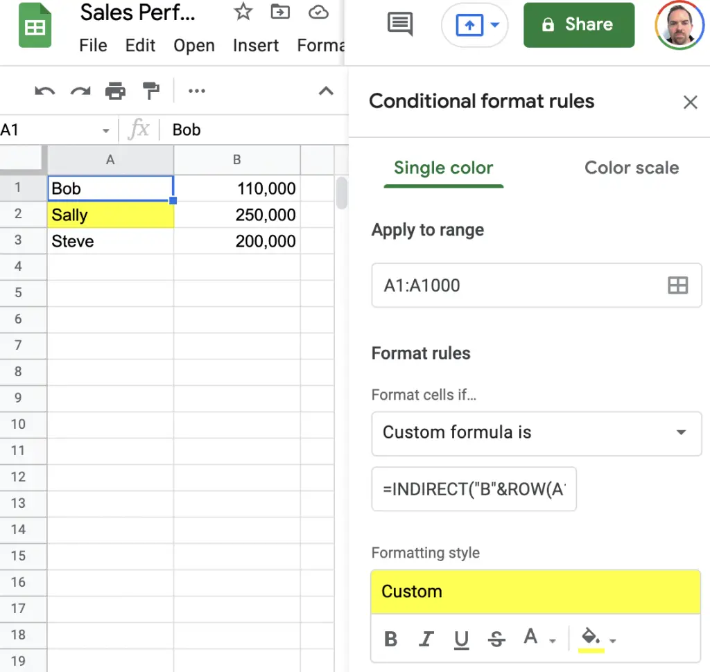
If you wanted to highlight the name of the staff member who had sold more than 200,000 you could use a Custom Formula on column A. Upon selecting all the cells you want the Conditional Formatting to apply insert the following formula:
This formula uses the handy INDIRECT() formula and starts by using the column name "B" where the information is stored to compare and then joins it to the corresponding cell used by Google Sheets in the range for the conditional formatting to be applied. As the range is A1:A1000 Google Sheets will replace this cell with each cell in the range.
Here’s how this looks:
You could further change the formula by creating another cell and setting the Named Range of that cell to salesTarget then your Custom Formula in the Conditional Formatting could reference an additional cell:
The important thing to remember when inserting a Custom Formula into the conditional formatting section is that there can only be one cell reference and this must be within the range to whom the formatting is applied.
Google Sheets Relative Referencing With Conditional Formatting
The INDIRECT() formula can also take relative references. Instead of using "B"&ROW(A1) you can also use the distance in rows or columns a range is from the active cell. This technique is known as relative referencing.
To use relative referencing in the INDIRECT() formula simply insert the relative reference using the distance in rows and columns away from the active cell.
For example, if the active cell were A1 and you were to use the INDIRECT formula with the relative reference of R1C1 in the active cell, this relative reference would increase the row by 1, and increase the column by 1. Therefore, this relative reference would copy the contents of cell B2.
To use the same row as the active cell don’t insert any numbers after the R tag in the relative reference.
Therefore, continuing with the example above, instead of using INDIRECT("B"&ROW(A1)) in the custom conditional formula, you could substitute this with the relative reference:
Notice with the first instance of the INDIRECT formula in the above condition that the parameters used in this formula have changed to RC1 and a second parameter FALSE has been added to assert that the indirect formula reference is a relative reference that does NOT use A1 notation (by default this parameter is set to TRUE).
Depending on your use case and which you prefer to use, relative referencing can just as easily be used and swapped out for A1 type referencing when using the INDIRECT() formula.
Conditional Format Custom Formulas: Common Errors
If you find your formula isn’t highlighting the right cells after you’ve entered your new Custom Formula there are a couple of things to check:
1. Is the formula correct?
Test your formula by inserting it somewhere on your sheet and seeing if it does work. In the case of the example above with the Sales staff I copied the formula into an adjacent column and checked to see if it would work, and it’s very easy to do, as shown below:
| A | B | C | |
|---|---|---|---|
| 1 | Bob | 110,000 | FALSE =INDIRECT("B"&ROW(A1))>200000 |
| 2 | Sally | 250,000 | TRUE =INDIRECT("B"&ROW(A2))>200000 |
| 3 | Steve | 200,000 | FALSE =INDIRECT("B"&ROW(A3))>200000 |
You should check your Custom Formula first to see if it will work.
Copy the same formula used in the Custom Formula into the top most cell and then copy this cell down checking that the cell reference (A1) changes too.
2. Is the cell reference in the Custom Formula “Apply to range” range?
Check the Apply to range field and verify the cell contained within your Custom formula will actually be found in that range.
For example, if the formula contained references to B1 instead of A1 (which is an easy mistake to make when you’re thinking about other columns!) then this will not work as anticipated.
3. Is the cell reference in the Custom Formula starting in upper-left-most range?
Check your cell reference in the Custom Formula matches the first cell range in the Apply To Range field. You can get strange behaviours if you use other cell references, so check the cell reference is the first cell in the range.
4. The background colour doesn’t match the conditional formatting set?
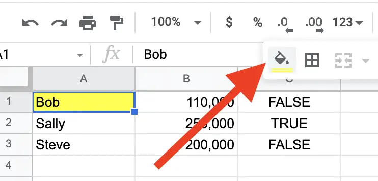
If you have a cell in your conditional format range that has a background colour not matching the rules of the format then this could be due to the cell’s background being set manually.
Simply look for the Fill Color icon and see if the background colour has a colour matching what you are seeing. If so, remove the background colour so that it doesn’t conflict with any conditional format rules you have set for the same range.
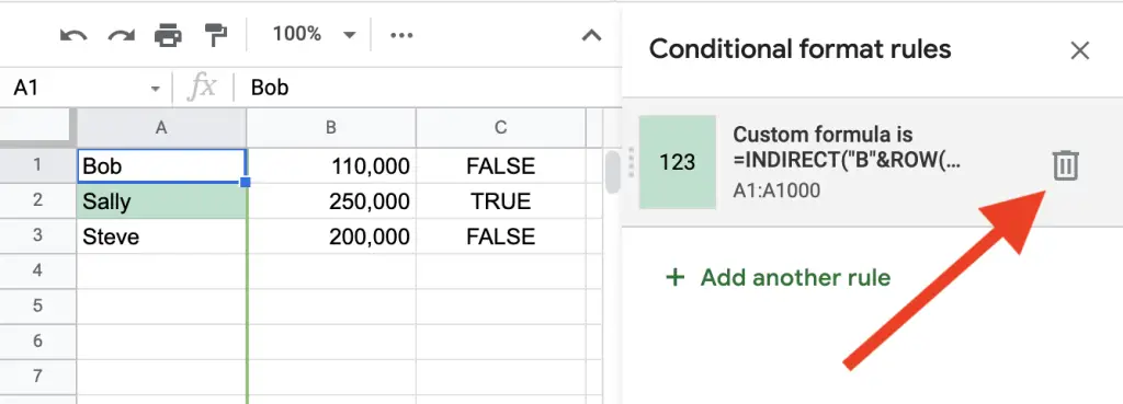
How To Remove Conditional Formatting
To remove a conditional format click first on a cell where you know formatting is applied, or, if in doubt, select all cells in the active sheet. Then click on the Format menu item followed by the Conditional formatting sub-menu item.
This will bring up a sidebar of the conditional formats available for either the selected cell or all cells you have selected.
To remove the desired condition simply hover your mouse over the row containing the formatting rules and you will see a rubbish bin icon appear and a tooltip will pop up stating Remove rule. To remove the rule simply click this button and the rules for the format will be deleted.
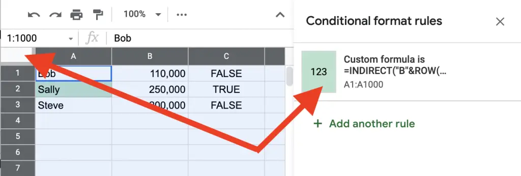
If you can’t find a conditional format rule try selecting all cells in the active sheet (click that grey box which doesn’t have any letters or numbers in it – it’s found to the left of label A for column A, and above label 1 for row 1). Here’s what this looks like when you do:
Summary
To enable references in the Custom Function field in the Conditional Formatting section of Google Sheets, insert either the reference or the Named Range into the INDIRECT() function.
The reason why the INDIRECT() function is needed is that only one cell reference can be used in the formula for Google Sheets to replace and apply the formula to other cells in the conditional formatting range.