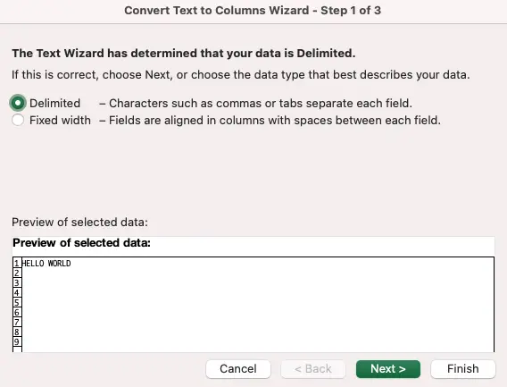
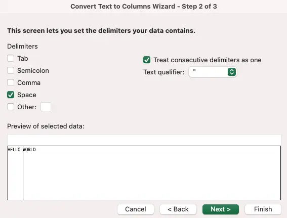
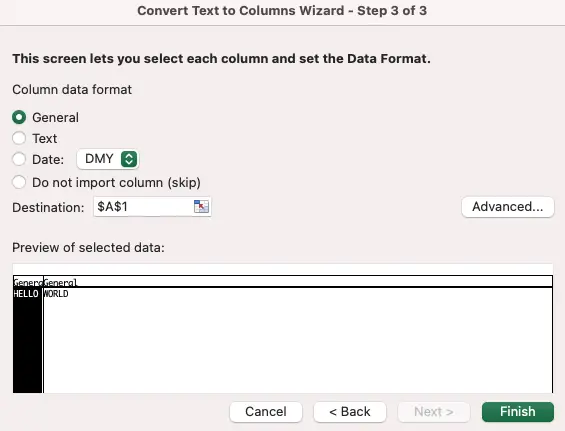
If a cell contains words it can be easy to split these into individual cells using the Text to columns feature in Excel. Simply select the cells you want to split into multiple columns, navigate to the Data menu then click on the Text to Columns button. From this Text Wizard window select Delimited width (click Next >), then set the delimiter type to Space (click Next >) then click Finish.
Here are the windows from the Text to Columns Wizard:
If you’re using a Google Sheets spreadsheet you can simply use the SPLIT function, like so:
| A | B | |
|---|---|---|
| 1 | HELLO WORLD | |
| 2 | HELLO =SPLIT(A1," ") | WORLD |
SPLIT enables you to split words into multiple cells
But how do you separate each character in a cell into individual cells?
To separate each character in the source cell ($A$1) into multiple cells use the MID function like so in an adjacent cell, like $B$1: MID($A$1, COLUMNS($A$1:A1), 1) and copy this formula across so that all characters from the source cell are separated into their individual cells.
What Does The MID Function Do?
The MID function takes three parameters, and has the following signature:
The first parameter takes a value, such as a string or a number to operate on. The second parameter is where to start capturing with 1 representing the first character from what was used in the value parameter. The third parameter is the number of characters to capture from the start value.
For example, MID("Hello World", 4, 1) would return just the 4th character l (as the length of the capture is just 1 character). If the formula were MID("Hello world", 4, 2) it would return lo (as the length of the capture is 2 characters).
Therefore, to extract each letter into its own cell would mean the MID formula would be capturing one character at a time. This would further mean the length property would be of value 1 and the start value would start at 1 and stop when it had progressed through the entire length of the cell.
Here’s an example:
| A | B | C | |
|---|---|---|---|
| 1 | HI | ||
| 2 | H =MID($A$1,1,1) | I =MID($A$1,2,1) | =MID($A$1,3,1) |
Using the MID formula multiple times enables capturing each character from the original word
Notice also from the above spreadsheet that if you try to capture an element that isn’t present in the cell, such as the third character from the word HI (there is none) it doesn’t error or throw an #N/A.
Two of the MID parameters are static: the first parameter references the cell to separate into individual cells, and the last parameter is just 1. So how can you make the second parameter more dynamic?
By using the COLUMNS formula you can capture the right index of the character needed according to its position, something like so:
| A | B | C | |
|---|---|---|---|
| 1 | HI | ||
| 2 | H =MID($A$1,COLUMNS($A$1:A1),1) | I =MID($A$1,COLUMNS($A$1:B1),1) | =MID($A$1,COLUMNS($A$1:C1),1) |
By using the COLUMNS formula for the second parameter as the formula is expanded left it will naturally capture the characters from the original cell
Separate Characters in Cell: Summary
The MID formula enables users to capture a minimum of one character from a reference cell. By using the MID($A$1, COLUMNS($A$1:A1), 1) formula and copying this across (to the right) you can have all characters in the original cell A1 separated into individual cells.
This same technique can apply to both Microsoft Excel spreadsheets and Google Sheets as the MID formula is common to both platforms.