I was recently working with a lot data on my Google Sheets spreadsheet and as I scrolled down the page the information from the top rows moved off and I could no longer see (and could no longer remember) what each column’s label in the first row was.
Thankfully there’s a nifty little feature in Google Sheets where you can freeze a set number of rows to lock the screen from moving as you continue to scroll down the page.
To create a header row quickly in Google Sheets click on the View menu item, then on Freeze and then select the best option presented: “No rows” (this removes any frozen rows), “1 row” (to freeze the first row), “2 rows” (to freeze the first two rows), “Up to current row” (freezes where you cursor is on the active sheet).
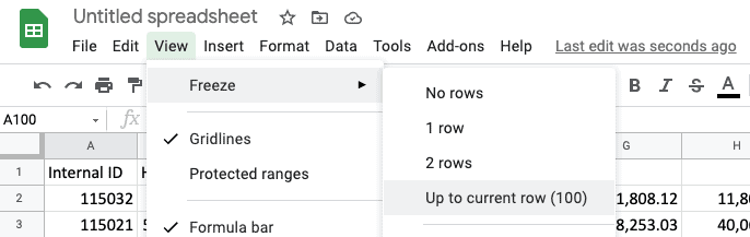
Easiest way to create a header row is from the main menu: click View, then Freeze, then select the desired rows to freeze
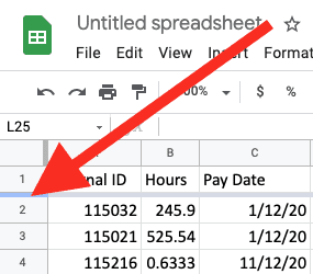
Another method of freezing your rows is by using your mouse cursor. If you hover your cursor to the top left-most grey cell, the one that is to the left of A column, and above row 1 (it doesn’t have any label in it’s box), as you move your mouse cursor to the lower border of that box you will see your cursor change from a pointer to a hand.
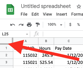
When your cursor is a hand you have the ability to click and drag this grey line down and as you move your mouse cursor down you will see a horizontal line extend across your sheet. This will give you the perspective on what rows will be frozen when you release your mouse button.
Another nifty feature of having frozen rows is that you can not only use these features for scrolling on your screen, but can also have these rows printed on your reports at the top of each page.
Print Header Rows In Google Sheets
Besides this tip being handy when navigating through each of your Google sheets another great feature of having frozen rows in your sheets is you can have them be printed at the top of each page.
This will help any person reading your reports as they scour through each page trying to remember what each label for your data set represents.
To make header rows available when printing your data, click on File, then Print, then open the Headers & footers item on the sidebar, and ensure the checkbox in the Row & column headers section labelled Repeat frozen rows is ticked.
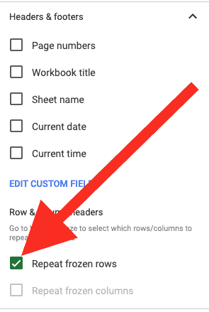
Then in the preview area of the document you are about to print you will see the header row repeated at the top of each page.
Completely Frozen Screen
If you want to prank your friends so that they are prevented from even scrolling up and down on their current active sheet set the cursor somewhere well below the active screen’s row depth. Say at row 100. Then from the View > Freeze menu item select the option “Up to current row (100)”.
You will know you’ve done it correctly when you see a warning box that states:
The current window is too small to properly display this sheet. Consider resizing your browser window or adjusting frozen rows and columns.
GOOGLE SHEETS WINDOW POP-UP
You can confirm everything has been frozen, because when you place your mouse cursor over the active sheet area you will not be able to get the sheet to scroll up or down at all! Even if you move your active cell using the arrow keys on the keyboard you will be unable to change the position of the active screen from the 100 frozen row view!
If you’ve been pranked or you’ve accidentally frozen your entire spreadsheet screen you’ll need to know how you can unfreeze your frozen sheet.
How To Remove Frozen Rows
The easiest way to remove a frozen row in Google Sheets is to click on the View menu item, click on the Freeze sub-menu item, and then click on the option labelled “No rows”. When this is clicked any frozen rows in your active sheet will automatically be removed.
Another way to similarly perform the same task using your mouse is to hover your mouse cursor over the thick grey line anywhere in your sheet and when your cursor changes from a pointer to a hand simply click and drag the thick grey line back to the top.
Summary
Freezing rows in Google Sheets is an easy way to keep labels of your columns available in your active view. If you’ve frozen too many rows, or have a completely frozen Google Sheet screen, then you can just as easily unfreeze any rows by using the View > Freeze menu items.
Check out our other article on how to do the same thing by locking columns in Google Sheets.