Flip ARRAY_CONSTRAIN Formula in Google Sheets (Example)

Previously I posted how you can use the INDEX() function to obtain the fields needed for a simple SUM() function.

Then I came across another handy Google Sheet function ARRAY_CONSTRAIN() .

What ARRAY_CONSTRAIN Does

There are three parameters with this formula:

1. range – insert the range for the formula to operate on.
2. num_rows – set the number of rows to compress.
3. num_cols – set the number of columns to compress.

All are required fields.

ARRAY_CONSTRAIN Example

Let’s look at a current depreciation problem I’m trying to solve.

I’m trying to compress the different types of depreciation on an array of different purchases projected over the next few years and to calculate what the new depreciation would be once these items have been purchased.

The data looks like this:

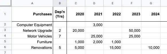
What we’re trying to achieve is to determine what the depreciation would be each year according to the year when items have been purchased, and their corresponding depreciation life in years.

Limitations of ARRAY_CONSTRAIN

Unfortunately the big limitation of ARRAY_CONSTRAIN is it works from the top-leftmost corner to cut the excess cells.

For example, if we apply the following formula on our data set:

=ARRAY_CONSTRAIN(C1:G6, 3, 2)

It will return for us the following highlighted cells:

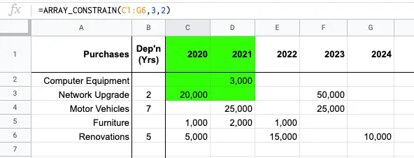
This causes a problem for our depreciation schedule as we’d like to fetch the last two years when we’re in the 2024 column for row 3, so using the following formula:

=ARRAY_CONSTRAIN($C3:G$3, 1, B$3)

For the Network Upgrade row would only return [20000,<blank>] , as these are the nearest to the top-left cells.

Workaround to ARRAY_CONSTRAIN

Is there a way to flip the input row?

There is!

Is there a REVERSE() function in Google Sheets we can apply to the range?

Unfortunately not yet.

So what we need to do as a workaround is to create our own REVERSE() function by sorting our data and reversing it backwards.

Thankfully my data already has a year row ( Row 1 ), all I need to be able to do is sort the data set by that row, apply descending sort and then insert the new range back into the ARRAY_CONSTRAIN() formula.

Here’s how I flipped my data range:

=ARRAY_CONSTRAIN(QUERY(TRANSPOSE($C$1:G3),"SELECT Col" & ROWS($C$1:G3) & " ORDER BY Col1 DESC", 0),$B3,1)

Let’s break apart this function and understand what’s happening, as usual we’ll start with the innermost functions and work out way out:

• ROWS($C$1:G3) – I used this to be able to get the column number to return from the QUERY function. As the last Column in the data set is the one I wanted, I just obtained this from the height of the original input range.
• TRANSPOSE($C$1:G3) – as my data set is in rows, I need to translate this into columns for it to be functional as a data set with the QUERY() function. The data set needs to include the row containing the years.
• QUERY(..., "SELECT Col" & ... & " ORDER BY Col1 DESC", 0) – the second SELECT parameter to our QUERY() function fetches just the one column, but orders by the first column being the column containing all the year values. The third parameter 0 just makes sure we don’t return any header rows.
• ARRAY_CONSTRAIN(..., $B3, 1) – we finally wrap everything back into our original ARRAY_CONSTRAIN function. This time we change the parameters a little as they are in a column format, but the purposes are still the same – we want the nearest 2 years (the value of cell $B3 ) – and as there’s only 1 column our third parameter is 1 .

To calculate depreciation on this row our final touch is to sum everything returned from the range and divide by the number of years:

=SUM(ARRAY_CONSTRAIN(QUERY(TRANSPOSE($C$1:G3, "SELECT Col" & ROWS($C$1:G3) & " ORDER BY Col1 DESC", 0), $B3, 1))/$B3

We further wrap the formula in a check to see if there are any depreciation values in the Dep’n (Years) column:

=IF(LEN($B3),SUM(...),"")

Result

Here’s the final result showing the function as well as our accumulated depreciation for the items purchased:

ARRAY_CONSTRAIN Summary

In this post, you’ve been able to discover and learn about the ARRAY_CONSTRAINT . You’ve seen its limitations in fetching from the upper-leftmost corner, and perhaps in time, Google Sheets will append an additional parameter to set where the corner should be fetched from.

In the meantime, we’ve discovered how we can reverse or flip a range to make use of the ARRAY_CONSTRAINT function by using the TRANSPOSE and QUERY functions together.