Google Sheets Named Functions In 5 Minutes

What is a named function in Google Sheets and when is it best to use this new feature in your spreadsheet?

Google Sheets new Named Functions feature enables you to refactor long formulas into what appears as a native function in your Google Sheets spreadsheet.

Use this feature in Google Sheets if you find you are using a complex formula more than once within your Google Sheets.

A recent need I found was with a finance spreadsheet which helped to calculate the right amount of tax to withhold. The original formula referenced a tax table that provided the variables to complete a linear function.

Here is what the tax table looked like on a sheet labelled TAXES :

	A	B	C
1	Weekly Earnings Less Than (x)	A	B
2	359	0	0
3	438	0.1900	68.3462
4	548	0.2900	112.1942
5	721	0.2100	68.3465
6	865	0.2190	74.8369
7	1,282	0.3477	186.2119
8	2,307	0.3450	182.7504
9	3,461	0.3900	286.5965
10	>3,461	0.4700	563.5196

Tax tables to help calculate the amount of tax to withhold

From this table I would then calculate my weekly earnings and use the following formula to calculate how much would be withheld from my pay each week:

=ROUND((TRUNC(INDEX(B:B,MATCH(1000,A:A,1)+1)*1000)+0.99)-INDEX(C:C,MATCH(1000,A:A,1)+1))

The above function searches for the weekly amount, in this case, 1000 in the first column and when it finds the corresponding match, it adds one to increase the row value so that it references the correct details. The INDEX function then uses this row reference to obtain the values for A and B to complete the linear function.

As this formula is used multiple times in my personal finance spreadsheet using the new Named Function feature in Google Sheets enabled me to refactor it so that it appeared as follows in the cells where this formula was contained:

=INCOME_TAX(A1,TAXES!A:A,TAXES!B:B,TAXES!C:C)

As you can see, the new Named Function is a lot more succinct than the previous formula!

Here’s how this Named Function was created.

Create A Named Function

To create a named function, simply click on the Data menu and then click on the Named Functions item. This will open a sidebar panel where you will need to enter the vital inputs.

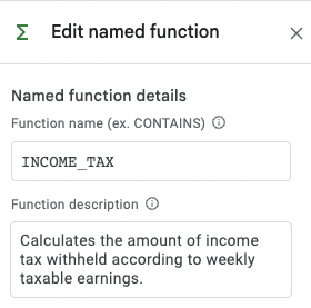
There will be an array of fields to complete with the first being the name of the function. In my case I entered INCOME_TAX (easy enough!).

Named functions are in capital letters and it may be more human-readable to use the underscore _ character between words.

Then in the next field labelled Function description I entered some detail about what the function outputs:

Calculates the amount of income tax withheld according to the weekly gross income and tax rates.
My function description

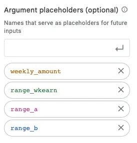
Start creating your named function by giving it a name and some details

Next is the field where you create the parameters to your function. This would be all the values you would need to enable your function to output a result.

In my case I needed the following inputs, which I created as follows:

weekly_amount
range_wkearn
range_a
range_b

The order here is important as this is how you’ll be inserting the values into your function. If you have optional parameters, put them at the end of your parameter declarations. Also, you cannot use upper case characters when creating your parameters, so space them out with underscores _ as I have done if needed.

You can also rearrange the order of the parameter fields by simply dragging and dropping them around in the order they need to go.

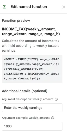
Create your parameters and put them in the right order

The next field labelled Formula definition where you can insert your original formula, but replace the values used in your original function with the corresponding labels created above.

Therefore, my formula definition has changed to the following:

=ROUND((TRUNC(INDEX(range_a,MATCH(weekly_amount,range_wkearn,1)+1)*weekly_amount)+0.99)-
INDEX(range_b,MATCH(weekly_amount,range_wkearn,1)+1))

Notice that the bones of this formula are still the same, I’ve just swapped out the input values and ranges/cell references to match the parameters.

Once you’re done, click on the Next button to proceed to the last step.

Document Your Parameters

The final step in creating your function is to provide a brief description of the parameters of your formula to help describe what type of input is required.

You should see a series of two fields per parameter defined in the previous screen. The first parameter enables you to enter a description about what is required for the parameter and the second is an example of the type of input needed.

For example, with the weekly_amount parameter I entered the following details:

Argument description: Enter the weekly earnings
Argument example: 1000

And for another parameter that I labelled range_wkearn I entered the following details:

Argument description: Enter the range of weekly earning tax tables
Argument example: B1:B100

Enter the parameter details for each argument created in the previous step

Then click Finish and you’ve successfully created your first named function in Google Sheets!

Using Named Functions In Your Spreadsheet

The next part is perhaps the easiest and this is where you can insert the function into your Google Sheet and use it like you would normally otherwise do just like any other standard function in Google Sheets.

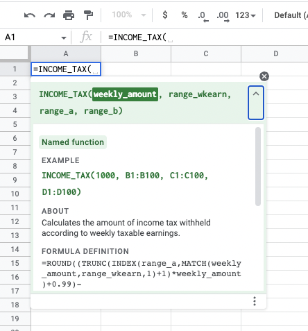
As I type the formula =INCOME the following bubble appears beneath my active cell:

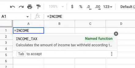
Start typing your new Named Function and you should see it pop up underneath your active cell

Upon confirming the function you can then click on the ? help icon to the right of the function declaration in your active cell and open up the documentation as you’ve typed previously.

My Named Function looks like this:

Your **Named Function** complete with your own documentation

This all goes to make the Named Function look and feel like a native Google Sheet function, which is amazing! And also helps in maintaining your big formulas by having one place to modify it.

Editing Named Functions

If you ever need to edit a named function already created simply click on the Data menu and Named Functions menu item and from the sidebar click on the three dots beside your named function and click Edit .

You can edit all aspects of your Named Function and the beauty is that it will automatically roll out to all instances within your active Google Sheet where the function is used.

For example, I initially labelled by Named Function PAYG_TAX but after changing the name to INCOME_TAX it automatically applied the change to every cell where I used the Named Function.

The same also applies to the function definition where if you find a faster or more efficient way of processing the information you can simply change the formula and it will automatically apply to wherever the formula is used.

This presents a powerful feature within Google Sheets that should make maintaining long formulas easy.

Summary

The Named Function in Google Sheets is a way to create your own custom functions within Google Sheets that make the function operate and feel like a native function.

The Named Function feature can enable you to more easily manage larger functions within your Google Sheets spreadsheet as well as provide documentation on what you’re trying to achieve.