Excel HLOOKUP Examples With Tips And Tricks

How do you use the HLOOKUP function in Excel properly and effectively?

As someone who frequently uses Excel, I understand how important it is to master various functions and features to enhance productivity and effectiveness. One such function that can be incredibly useful when working with large data sets is the HLOOKUP function.

In this article, I’ll share a few examples to demonstrate how this function can improve your data analysis skills.

For those unfamiliar with the HLOOKUP function, it stands for Horizontal Lookup . This function searches for a specified value in the top row of a table or an array of values and then returns the corresponding value in a specified row within the table. It can save time and effort, especially when comparing or retrieving data from different sources or spreadsheets.

What Is HLOOKUP?

As a regular user of Excel spreadsheets, I often encounter situations where I need to search for specific information within a sheet. One useful function that helps me with this task is HLOOKUP and I find this function particularly helpful when obtaining data from a specific year for an item.

Most data sets I handle are financial, with the top horizontal axis representing the year, so if I need to calculate rates based on the number of sales and total sales of a product in a particular year I have found the HLOOKUP function a handy formula to use.

Excel HLOOKUP Syntax

The Horizontal Lookup function is a powerful spreadsheet function that allows you to search for data in horizontal rows, based on a specific reference value.

The syntax for the HLOOKUP function is as follows:

=HLOOKUP(lookup_value, table_array, row_index_num, [range_lookup])

Here’s a brief explanation of each argument:

• lookup_value : This is the value you want to search for within the table_array .
• table_array : The table range where you’ll be searching for the lookup_value . This is typically a set of rows containing data.
• row_index_num : The row number you want to return the data from within the table_array . The first row containing the lookup_value represents 1 .
• range_lookup : This is an optional argument that specifies whether you want to enable an approximate match for the lookup_value . If set to TRUE or omitted, Excel will return an approximate match. If set to FALSE , Excel will search for an exact match.

HLOOKUP Examples

Suppose you have the following sheet with the following financial totals representing the Sales of each product per year, like so:

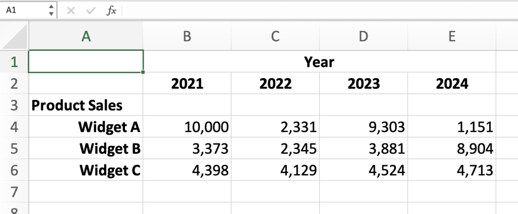
With this type of data set if I need to fetch the total sales for a particular widget according to year, then I can use the HLOOKUP formula as follows:

=HLOOKUP(2021,Sales!B2:E6,3,FALSE)

What will this formula return?

This formula will fetch the Sales in 2021 for Widget A.

• The lookup_value is the year 2021 .
• The table_array is the range Sales!B2:E6 .
• The row_index_num is the number 3 , representing the row B4:E4 .
• The range_lookup is FALSE , meaning an exact match of lookup_value ( 2021 ) needs to be found in the first row B2:E2 of my table_array .

Therefore, the HLOOKUP looks for 2021 in the range B2:E2 (which it finds in the first cell B2 ). With this value found, it then counts down 3 rows and returns the value 10,000 .

What would happen if some of the values in the above HLOOKUP formula were changed?

What would the following formula return?

=HLOOKUP(2023,Sales!B2:E6,5,FALSE)

What value did you get?

Stepping through this formula the answer you would get is as follows:

• Search for the value 2023 in the first row of the table B2:E6 .
• This value is found in cell D2 .
• From this cell count 5 rows with the current row in D2 being 1 .
• Therefore, the answer is the value found in cell D6 being 4,524.

This formula is therefore returning the total sales of Widget C in 2023.

Another HLOOKUP Example

Another way I have used the HLOOKUP formula is by obtaining specific assessment results of students.

Assume I have performed a few tests on my students and the results of these students are recorded below as follows:

	A	B	C	D
1	Student	Test 1	Test 2	Test 3
2	Alice	75	80	85
3	Bob	60	65	70
4	Charlie	90	95	100

If I want to find the score of Bob in Test 2 , I can use the HLOOKUP function like this:

=HLOOKUP("Test 2",A1:D4,3,FALSE)

The result will be 65 , which is Bob’s score in Test 2.

Advanced HLOOKUP: Tips And Tricks

When working with HLOOKUP in Excel there are a couple of things I am more aware of when using the formula than I would otherwise be when using VLOOKUP . And the biggest aspect is that the rows which search for the value I want may not be static.

Have a look at the following example with my original widget sale table, and watch how easy it is to break the original HLOOKUP formula:

There are a couple of ways I’ve circumvented these problems when dealing with HLOOKUP formulas.

HLOOKUP Returns Final Row

If the HLOOKUP formula will always return the last row in the formula, in the third parameter of the HLOOKUP function wrap the same table_array in the ROWS() formula.

=HLOOKUP(2021,Sales!B2:E6,ROWS(Sales!B2:E6),FALSE)

This helps, especially when more rows are likely to be inserted (or deleted) above the row you’re seeking to return.

Here’s how this would look if I my formula was seeking 2021 for Widget C with the above data:

Dynamic HLOOKUP Row

What if the row being returned can move? In this case, you would need to search for the row and have it return its location. For this use MATCH() like this:

=HLOOKUP(2021,Sales!B6:E6,MATCH("Widget C",A2:A6,0),FALSE)

Here’s how this formula looks:

Notice in the above when the actual row is moved it does cause the HLOOKUP any problems.

Common HLOOKUP Errors

Besides working around possible issues when dealing with HLOOKUP formulas, there are still common lookup errors that can also happen.

#N/A

This error occurs when HLOOKUP can’t find a match for the lookup value in the specified row. To fix this, double-check for typos or formatting disparities between the lookup value and the table array. Using the IFNA or IFERROR functions can help to display a specific message or value if there’s no match.

=IFERROR(HLOOKUP(value, table, row_index, TRUE), "Not Found")

Error	Description	Solution
#N/A	Lookup value not found	Double-check spelling and formatting. Wrap HLOOKUP in IFNA or IFERROR functions to mitigate problems if this formula is used in other formulas elsewhere.

#VALUE!

This error occurs when the row index number in HLOOKUP is less than 1, or not an integer.

To fix this, ensure that the row index number is a valid integer and greater than or equal to 1.

Error	Description	Solution
#VALUE!	Row index number invalid	Ensure row index number is a valid integer and greater than or equal to 1.

#REF!

This error occurs when the row index number in HLOOKUP is greater than the number of rows in the table array.

To fix this, review the table array and reduce the row index number accordingly.

If you want to know what the maximum number of rows available in your table_array use the formula ROWS(table_array) .

Error	Description	Solution
#REF!	Row index number out of range	Reduce the row index number to match the table array’s size.

Finally, it’s worth mentioning that using non-unique identifiers in the lookup row can lead to inaccurate results or the return of the first match encountered. To maximise the effectiveness of HLOOKUP , ensure that the lookup row contains unique values if the fourth parameter is set to FALSE (otherwise 0 will likely be the response).

HLOOKUP Examples: Summary

In this article, I’ve shared some examples of using the HLOOKUP function in Excel. Through these examples, I hope you’ve gained a better understanding of this useful tool and how it can help in various situations.

Finally, while HLOOKUP can be a valuable addition to your Excel toolkit, don’t forget to explore other functions and features Excel has to offer. There’s a wealth of tools available to make your work more manageable and help you analyse data more effectively. Happy spreadsheeting!