5 Ways To Alphabetize In Google Sheets (Examples With Screenshots)

How can you alphabetize or sort your data in Google Sheets?

There are 5 ways to alphabetize data in Google Sheets: two approaches involve using formulas; namely, the SORT() and QUERY() functions, and the other three approaches involve using the menu items located in the menu bar. All approaches require knowing if the sorting will be done in ascending order, where your data starts from those cells closest to A and ends with cells closest to Z, or in descending order which does the opposite.

For example, if your range contained the words Fred, Alice, Katie and Bob and you wanted this sorted in ascending order, any of the sort options would change that data to be arranged like this: Alice, Bob, Fred and Katie.

Here are some additional details on each approach, with examples and screenshots below.

Alphabetize Using Sort Menu Options

There are two available options when sorting data in Google Sheets: sort sheet and sort range.

Both items perform the same thing, however, if you want to sort a specific range on your sheet then you need to highlight the range first before choosing the menu item.

1. Alphabetize Entire Sheet

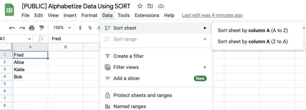
To sort an entire sheet, ensure the sheet you want to sort is active on your screen. Then click on the main menu item labelled Data , hover over the menu item Sort Sheet , then from the sub-menu items, select either Sort sheet by column A (A to Z) or Sort sheet by column A (Z to A) .

Here is what this menu looks like in Google Sheets:

According to the type of order sought, your data on the active sheet should modify accordingly.

However, note that this type of sort just looks at column A in the active sheet and sorts the entire sheet according to the contents in column A.

Here is the result of how the active sheet looks once the Sort sheet by column A (A to Z) looks like:

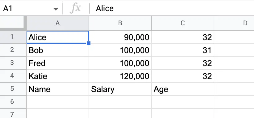
As you can see, the data did correctly sort everything by the contents in column A and kept all the rows aligned to their respective data. However, it didn’t consider the fact that the first row in the sheet was a header row and shouldn’t have been part of the sort.

How do you prevent the sorting feature from including the header row in your sort? This is where the next sort option comes in very handy: sorting by range.

2. Alphabetize By Range

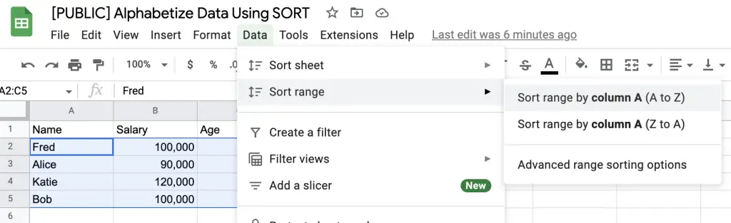
To alphabetize a specific range, you must select all the cells in the active sheet you want to sort. If you haven’t selected a range, you will be unable to select a range as the menu item will be greyed out, preventing you from proceeding any further. Therefore, if it is greyed out, highlight the range first and then select the Data main menu, followed by the Sort range menu item and then select Sort range by column A (A to Z) or Sort range by column A (Z to A) or Advanced range sorting options .

As I have the entire sheet highlighted, the sub-menu items may differ according to the range you have highlighted. For example, if you have highlighted columns B to D, the sub-menu would instead state Sort range by column B (A to Z) – whatever happens to be your first column in the range will be used as the column name.

The first two sub-menu options behave in the same way as above with sorting a sheet. It will sort according to the first column in your selected range. Therefore, to eliminate the problem of having the header row sorted, you could just select the range of data and then sort your data, like so:

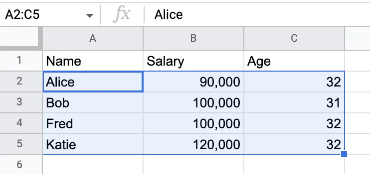
This produces the desired outcome of the data being sorted and not the header row, as shown below:

But what if you wanted to sort your data by another column instead of the first? This is where the advanced sorting option becomes a very handy sorting tool.

3. Alphabetize By Multiple Columns

To sort a range by anything but the first column or to perform multi-column sorts, the Advanced range sorting options provide an excellent means of achieving this feat.

To use this feature, highlight your range, and from the Data > Sort range menu item, select the option Advanced range sorting options, which will pop up a modal window over your active sheet like so:

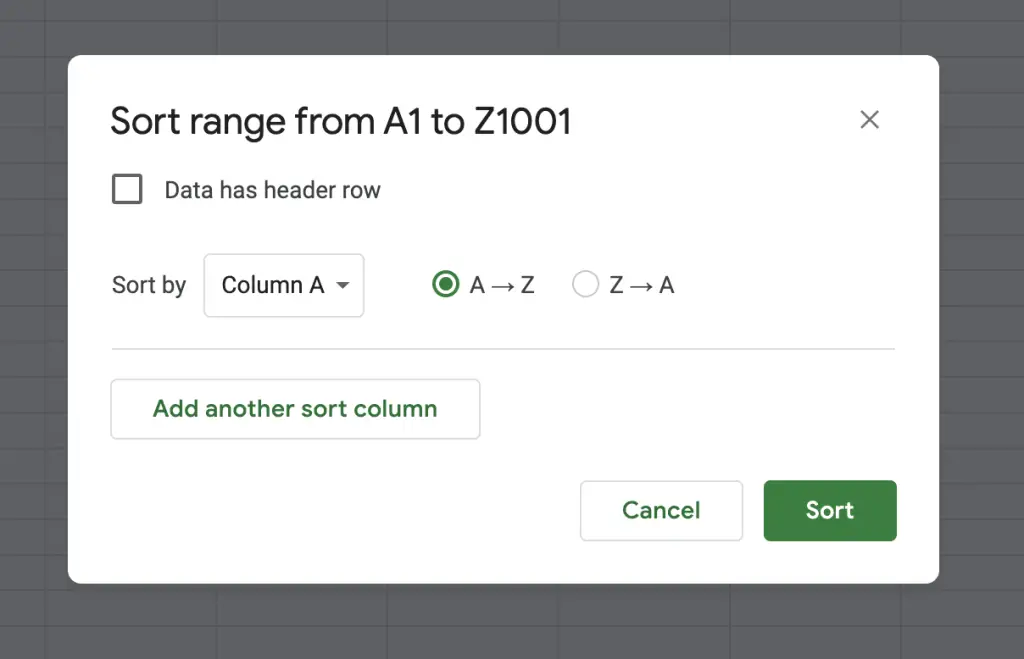
Here you will be presented with a few more options. The checkbox labelled Data has header row is important to select if your highlighted range includes the header row . If you select this option, the header row will not be included in the sort. Otherwise, if your range doesn’t include a header row, then leave this checkbox unticked .

As I had selected the entire sheet, my data includes a header row. Therefore, I will tick this box. If you do tick this box, the Column A labels in the drop-down menu underneath change to match the header row titles, as seen with my data here:

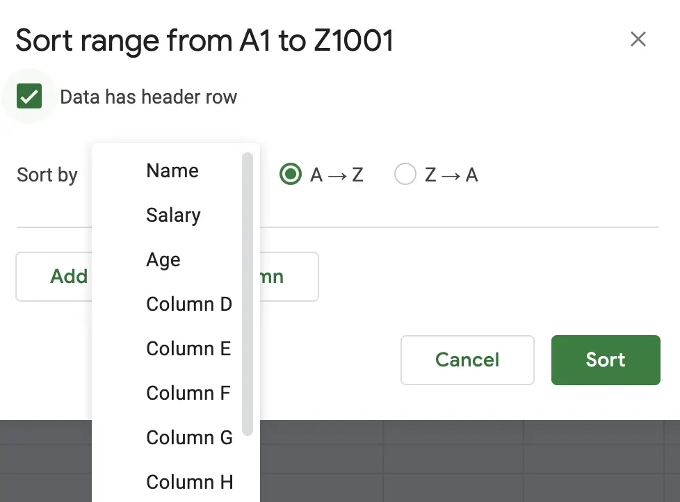
To perform sorting on any other column, I just select the drop-down item I want the data to be sorted by.

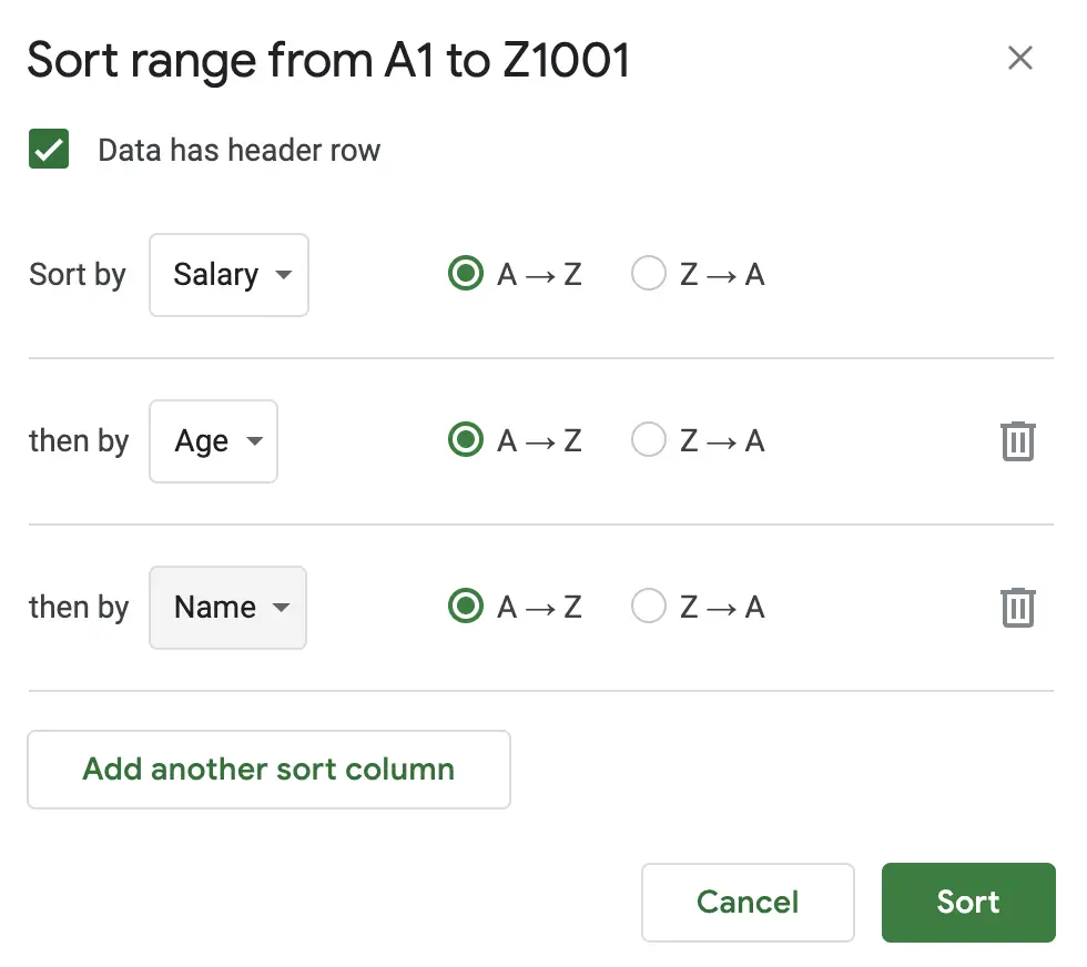
If you want to perform a sort using multiple columns, you can simply click on the Add another sort column and select the column to sort by. Using the example spreadsheet, if I wanted to sort by the Salary column, then by Age, then by Name, the structure would look like this:

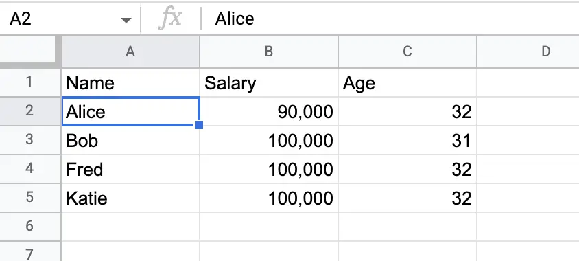
As you can see from the result, this produces a list with the lowest salary first. Then where salary figures are the same, such as with Bob, Fred and Katie, the Age column is used to sort who ranks higher than the other. In my case, Bob is the youngest and therefore ranks above Fred and Katie. Finally, the next criteria sorts those rows which have the same salary and same age by sorting those rows alphabetically by their name. As Fred and Katie share the same salary and age, Fred is listed higher due to his name being alphabetically first than Katie.

The Advanced sorting option for a range is one of the most common methods to sort in Google Sheets, and you will find yourself frequently using this the more you use spreadsheets.

Alphabetize Using Functions

Google Sheets provides two functions that enable users to sort their data: SORT() and QUERY() .

4. Alphabetize Using SORT() Function

Another way you can sort your data is by using the SORT() function in Google Sheets.

The SORT() function is more versatile because, just like the Advanced range options with sorting by range, you can use it to sort by multiple columns.

The syntax for the SORT() function is as follows: SORT(range, sort_column, is_ascending, [sort_column2, is_ascending2, ...]) where range is the range you want to sort, sort_column is the index of the column you want to sort or a range of the same height as range , and is_ascending which would be TRUE to sort the data in ascending order (from A to Z) or FALSE to sort in descending order (from Z to A). If additional columns are needed to perform the sort, append pairs of sort_column with is_ascending parameters.

Here’s how a simple sort would look if applying the sort on the entire data set and using just the first column as the sorting column. Here’s the formula, followed by the result:

=SORT(MultiColumnSort!A:C, 1, TRUE)

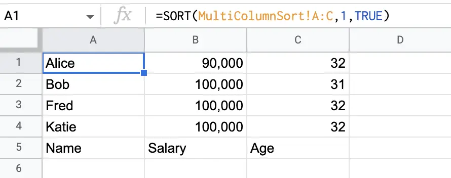
As you can see from the above result, the formula functions in the same way as options 1 and 2 do above. It doesn’t consider the header row in the range. Therefore, to make it function appropriately, you must exclude the header row from being used in the range .

If you want to output the header row in addition to the data, then check the next option by using the QUERY() function.

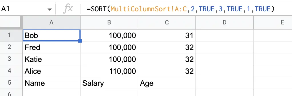
To use the SORT() function with multiple columns, append into the parameters of the SORT() function the column with ascending type. If you wanted to replicate the same result as shown in option 3 above, the formula would look as follows:

=SORT(MultiColumnSort!A:C, 2, TRUE, 3, TRUE, 1, TRUE)

This produces the following result, which is the same as option 3, except, once again, the header is also used in the sort:

As you can see from the examples above, a reason for not choosing the SORT() function is where the range includes the header row. The SORT() function works well on data without a header row and can perform multiple column sorting.

So how can you sort your data and notify Google Sheets that the first row includes a header row – this is where the powerful QUERY() function comes in.

5. Alphabetize Using QUERY() Function

The QUERY() function is a powerful formula that allows you to run database-like statements on your data. The syntax of the QUERY() function is: QUERY(data, query, header_rows) . The 3 parameters are data , which can be a range, query , which is the database-like statement, and an optional third parameter, header_rows , which lets the formula know how many header rows there are in the data.

Using the same data as the SORT() function did above to perform a simple sort would look something like this:

=QUERY(MultiColumnSort!A:C, "SELECT * WHERE NOT A = '' ORDER BY A", 1)

This formula produces the following result:

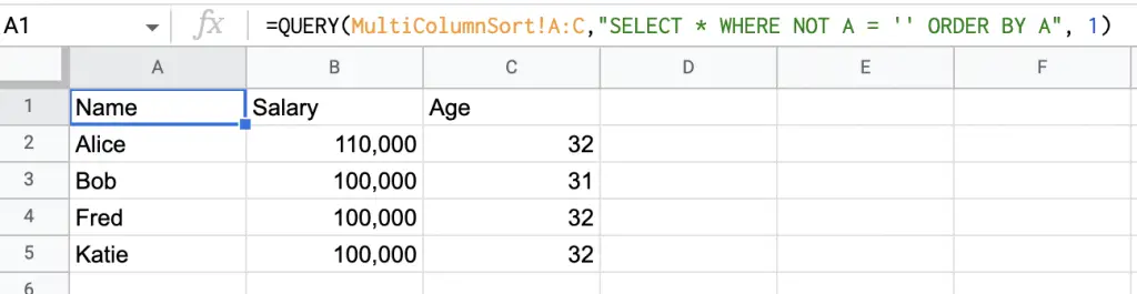
The query statement in the formula selects all data in the columns and where the data in column A is not empty (or blank) it will order the data alphabetically by column A. As the original data set contains 1 header row, I add the number 1 into the last parameter.

As you can see from the above, the result produced is precisely what was needed. The sorting aspect in the QUERY() formula happens in the ORDER BY statement, which takes a column name or ColX index number followed by ASC or DESC depending on how you want to sort the data.

For example, if you wanted to sort the data in descending fashion, then the formula would have looked like this:

=QUERY(MultiColumnSort!A:C, "SELECT * WHERE NOT A = '' ORDER BY A DESC", 1)

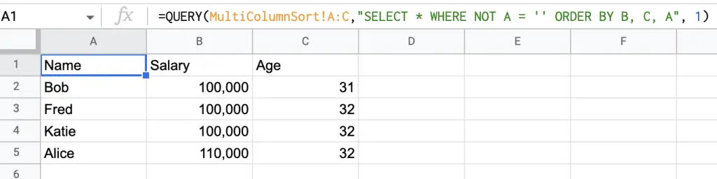
To perform multiple column sorting on your data separate each column sorting instruction by a column as follows:

=QUERY(MultiColumnSort!A:C, "SELECT * WHERE NOT A = '' ORDER BY B, C, A", 1)

Which matches the option 3 result:

The QUERY() function is a versatile function that provides the capacity of both inserting the header and performing multiple column sorting.

Summary

There are 5 ways in Google Sheets to alphabetize your data. Three methods are obtained from within the menu structure where 2 from the menu do the same thing by sorting based on the first column, whereas the Advanced sort option enables sorting on a range using multiple columns.

The other two ways in Google Sheets to alphabetize your data is to use functions: SORT() and QUERY() . If you’re using a range of data without a header row then you could easily use the SORT() function. However, if your data contains a header row and you want to retain this header row in your result then use the QUERY() function.

Both functions enable multiple column sorting. However, the QUERY() function is a more powerful option, provided you put the time into learning about the SQL-like syntax.