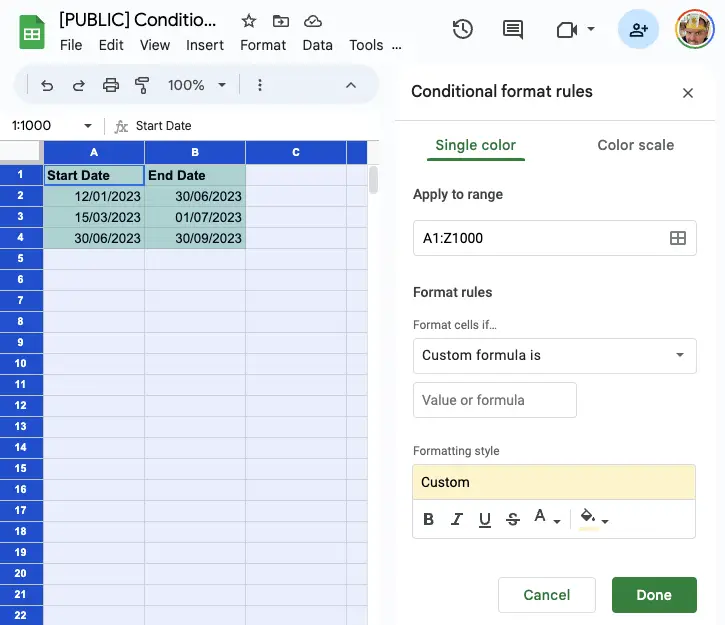
How can you highlight a column of dates based upon a condition where comparison is needed with the current column of dates to another column containing dates?
I had a requirement where I needed to compare a column of dates to another column of dates and if a specific date was between those dates to highlight one of the columns.
For example, I needed to highlight a cell when the start date and the end date crossed over the end of the financial year. As the end of the financial year in Australia is 30th June each year if the start date was before the 30th June and the end date was after the 30th June then I wanted to highlight the row.
The formula was easy enough as other posts have demonstrated how you can use the Conditional Formatting feature in Google Sheets along with a Custom Formula to generate all types of useful highlighting functions.
Here was the final formula:
And here’s what each of the functions within this formula mean, starting with the inner most functions:
INDIRECT("RC", FALSE) this function obtains the current cell when iterating through the Conditional Formatting range in the Google Sheet.
ROW(INDIRECT("RC", FALSE)) the ROW() function obtains the row number of the current cell. For example, if the current cell were A3 the row would be 3, if it were C45 it would return 45.
INDIRECT("A"&ROW(INDIRECT("RC", FALSE))) this creates a reference to the data contained in the Start Date column. For example, if the current cell was C4 the row formula would 4 and this would create the range "A4". With INDIRECT() wrapping around that reference Google Sheets would obtain the value in that cell, being 30/06/2023.
MONTH(INDIRECT("A"&ROW(INDIRECT("RC", FALSE)))) returns the month of the date in the cell being referenced.
AND(MONTH(INDIRECT(“A”&ROW(INDIRECT(“RC”, FALSE))))<=6, MONTH(INDIRECT(“B”&ROW(INDIRECT(“RC”, FALSE))))``>6) with the final function AND wrapping the check to see if both month values of the dates referenced have occurred either side of the month of June.
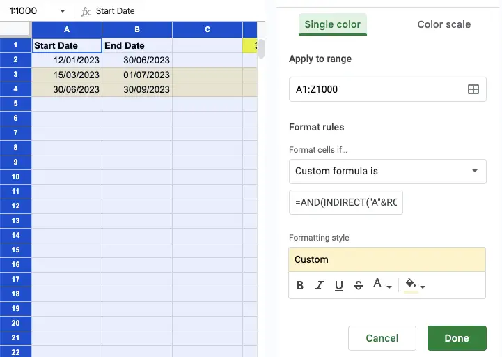
When pasting this formula into the Value or formula field, it will look like this:
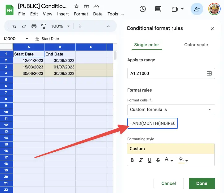
If you see a red outline around the Value or formula field then it means there is something wrong with your formula. Check you’ve inserted the right number of brackets!
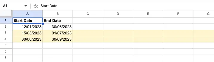
Once everything looks like it’s in working order click the Done button and you should see your rows highlighted according to your new conditional formatting.
Here’s how my sheet then looked:
Highlighting Based On Specific Date
While I made use of the MONTH() function to determine whether the two dates were on either side of a specific date, you could modify the formula to be more explicit on a date field.
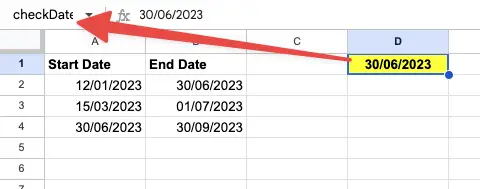
To modify the custom formula to work around a specific date, use a cell and name it according to your needs.
In my case I have used a cell and named it checkDate:
Then in the conditional formatting custom formula for the entire range in the sheet enter the following formula:
Here’s the formula to insert:
And the result is as follows:
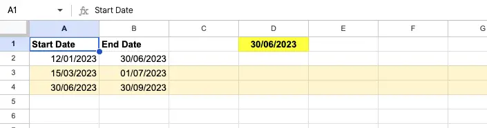
Notice the slight change to the formula. Instead of using the MONTH() function the comparison is to a named cell and to use that named cell it needs to be wrapped with INDIRECT().
Highlighting Rows Based On Date Cells In Row: Summary
To highlight an entire row based on the values of date cells in a common row use the INDIRECT() function along with the AND() function to create a formula that compares the cells containing your dates to the comparative date cell.
Other techniques you could use could be to compare the cells using date functions like the MONTH() function.
If you want to see more examples using the Conditional Formatting method with Custom Formulas check out this post.
If you wanted to check the Google Sheet out used in this post and make a copy for your own purposes, then you will find the Conditional Formatting Google Sheet here.